Hit the Hide Code button to hide the R code.
Synopsis
This workflow contains diversity assessments for the full data set—all replicate samples—and the merged data set—replicates combined by sample. In order to run the workflow, you either need to first run the DADA2 Workflow and the Data Preparation workflow or begin with the output files from the Data Preparation workflow. See the Data Availability page for complete details.
In this workflow…
Full Data Set (ASV)
Read Distribution
Histogram of Read Counts
ssu_max <- max(ssu_ps_samp_data$total_reads) +
  (0.2 * max(ssu_ps_samp_data$total_reads))
ssu_p_hist <- ggplot(ssu_ps_samp_data,
       aes(ssu_ps_samp_data$total_reads)) +
         geom_histogram(breaks = seq(0, ssu_max, by = 5000),
                        col = "black", fill = "grey") +
         labs(title = "Distribution of total reads (FULL)",
              caption = "Bin width equals 5000 reads") +
  labs(x = "No. of reads", y = "No. of samples") +
  theme_classic()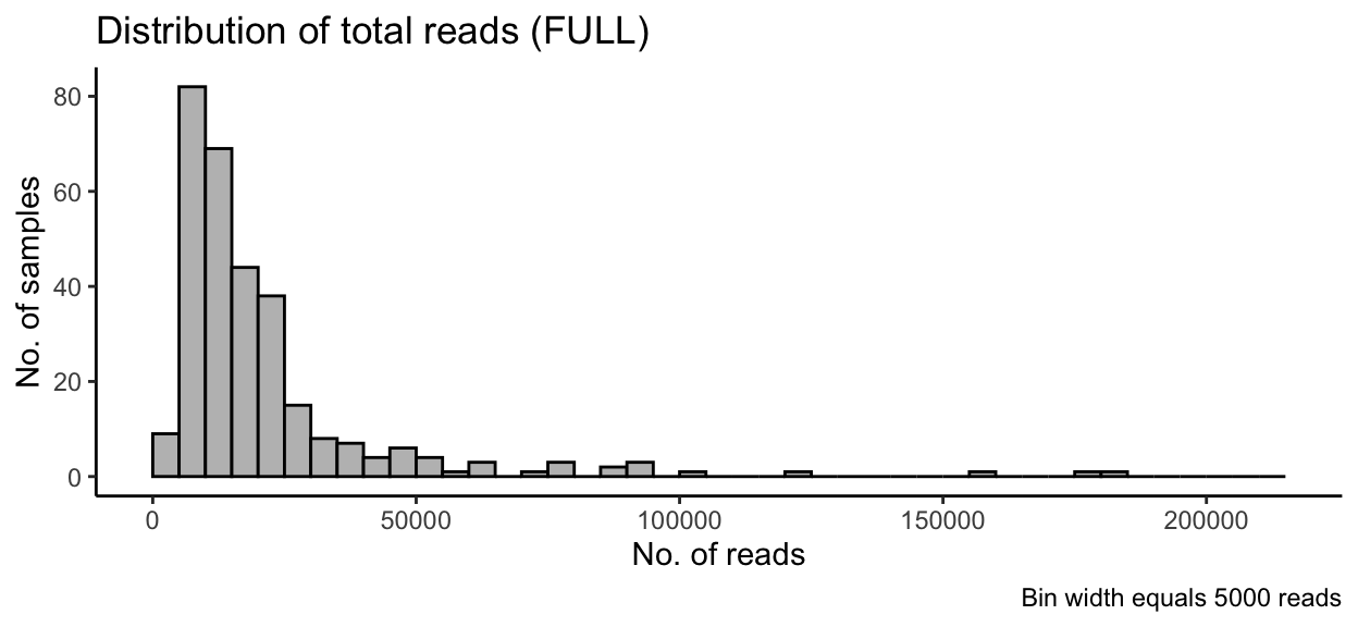
Rarefaction Curves
tmp_select <- ssu_amp_data
tmp_select$metadata$SITE <- factor(tmp_select$metadata$SITE,
                                   levels = c("ALMR", "PAST", "CRIS", "PUCL"))
ssu_rare_curve1 <- amp_rarecurve(
  tmp_select,
  stepsize = 1000,
  color_by = "SITE"
) + scale_colour_manual(values = swel_col)
ssu_rare_curve1 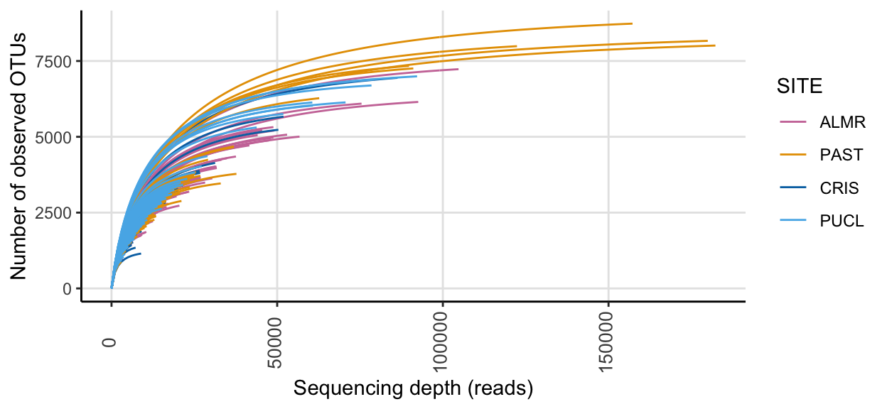
For a quick comparison, we can facet the above data by Site.
ssu_rare_curve2 <- amp_rarecurve(
  tmp_select,
  stepsize = 1000,
  color_by = "SITE",
  facet_by = "SITE",
  facet_scales = "free"
)  + scale_colour_manual(values = swel_col)
ssu_rare_curve2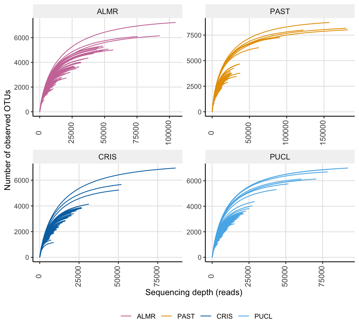
In the full data set, there was a minimum read count of 2699, a median of 13974 reads, and a maximum of 182257 reads. After PIME filtering, there was a minimum read count of 2027, a median of 2347.5 reads, and a maximum of 2482 reads.
Alpha Diversity
To account for presence of rare sequence variants caused by sequencing errors or other technical artifacts, we use Hill numbers (Alberdi and Gilbert 2019a). Hill numbers allow the weight put on rare versus abundant sequence variants to be scaled while providing intuitive comparisons of diversity levels using “effective number of ASVs” as a measuring unit. This approach allows for balancing the over representation of rare ASVs that might be inflated due to sequencing errors.
We will then use Shapiro-Wilk tests to test for normalcy and then, depending on the results, either use parametric ANOVA or non-parametric Kruskal-Wallis to compare alpha diversity among treatments.
Calculate Hill Numbers
To calculate Hill numbers, we use the R package hilldiv (Alberdi and Gilbert 2019b). We calculate three metrics that put more or less weight on common species:
- Observed richness, where
q-value = 0. - Shannon exponential, which weighs ASVs by their frequency, where
q-value = 1. - Simpson multiplicative inverse, which over weighs abundant ASVs, where
q-value = 2.
We perform each analysis against the full data set and the PIME filtered data set using the function hill_div.
The command is as follows:
hill_div(count = x, qvalue = i, tree = ultrametric_tree), where x is the sample by ASV table, i is the q-value corresponding to the metric of interest and tree is an ultrametric formatted phylogenetic tree (see below).
We first transform all the data to relative abundance values, and compute new trees.
ssu_alpha_ds <- c("ssu_ps_work", "ssu_ps_pime")
objects()
for (i in ssu_alpha_ds) {
tmp_ps <- transform_sample_counts(get(i), function(otu) otu/sum(otu))
tmp_ps@phy_tree <- NULL
tmp_tree <- rtree(ntaxa(tmp_ps), rooted = TRUE,
tip.label = taxa_names(tmp_ps))
tmp_ps_norm <- merge_phyloseq(tmp_ps, sample_data, tmp_tree)
tmp_asv <- data.frame(t(otu_table(tmp_ps_norm)))
tmp_ps_name <- purrr::map_chr(i, ~ paste0(., "_norm"))
assign(tmp_ps_name, tmp_ps_norm)
tmp_asv_name <- purrr::map_chr(i, ~ paste0(., "_tu"))
assign(tmp_asv_name, tmp_asv)
rm(list = ls(pattern = "tmp_"))
}No phylogenetic tree
Next, we run the analysis for all three metrics on the data sets without a tree.
qvalue <- c(0,1,2)
for (i in qvalue) {
  for (j in ssu_alpha_ds) {
     tmp_asv <- get(purrr::map_chr(j, ~ paste0(., "_tu")))
     tmp_df <- data.frame(hill_div(tmp_asv, qvalue = i))
     tmp_df <- tmp_df %>% dplyr::rename("tmp_name" = 1) %>%
                              tibble::rownames_to_column("SamName")
     tmp_name <- purrr::map_chr(j, ~ paste0(., "_h", i))
     print(tmp_name)
     assign(tmp_name, tmp_df)
     rm(list = ls(pattern = "tmp_"))
  }
}
objects(pattern = "_h")
And make summary tables to add back into each ps object.
for (i in ssu_alpha_ds) {
     tmp_obs <- get(purrr::map_chr(i, ~ paste0(., "_h0")))
     tmp_sha <- get(purrr::map_chr(i, ~ paste0(., "_h1")))
     tmp_sim <- get(purrr::map_chr(i, ~ paste0(., "_h2")))
     tmp_hill <- dplyr::left_join(tmp_obs, tmp_sha, by = "SamName") %>%
       dplyr::left_join(., tmp_sim, by = "SamName") %>%
       dplyr::rename("Observed" = 2, "Shannon_exp" = 3, "InvSimpson" = 4)
     tmp_name <- purrr::map_chr(i, ~ paste0(., "_hill"))
     assign(tmp_name, tmp_hill)
     rm(list = ls(pattern = "tmp_"))
}
objects(pattern = "_hill")
And then create the new objects with the diversity data.
With a phylogenetic tree
We can also run the tests using the phylogenetic tree to assess lineage diversity rather that ASV diversity for the PIME data set. For this part we will only use PIME filtered data sets. We do a quick check to ensure the ASV names in the ASV table and the tip names in the new phylogenetic tree are identical.
ssu_alpha_ds_tree <- c("ssu_ps_pime")
qvalue <- c(0,1,2)
for (i in qvalue) {
  for (j in ssu_alpha_ds_tree) {
     tmp_asv <- get(purrr::map_chr(j, ~ paste0(., "_tu")))
     tmp_tree <- get(purrr::map_chr(j, ~ paste0(., "_tree_ult")))
     tmp_df <- data.frame(hill_div(tmp_asv, qvalue = i, tree = tmp_tree))
     tmp_df <- tmp_df %>% dplyr::rename("tmp_name" = 1) %>%
                              tibble::rownames_to_column("SamName")
     tmp_name <- purrr::map_chr(j, ~ paste0(., "_ht", i))
     print(tmp_name)
     assign(tmp_name, tmp_df)
     rm(list = ls(pattern = "tmp_"))
  }
}
objects(pattern="_ht")
save(ssu_ps_pime_ht0, ssu_ps_pime_ht1, ssu_ps_pime_ht2, ssu_ps_pime_merge_ht0,
     ssu_ps_pime_merge_ht1, ssu_ps_pime_merge_ht2,
     file = "files/trepo/alpha/rdata/ssu_ps_pime_hill_tree_tests.rdata")
for (i in ssu_alpha_ds_tree) {
tmp_obs <- get(purrr::map_chr(i, ~ paste0(., "_ht0")))
tmp_sha <- get(purrr::map_chr(i, ~ paste0(., "_ht1")))
tmp_sim <- get(purrr::map_chr(i, ~ paste0(., "_ht2")))
tmp_hill <- dplyr::left_join(tmp_obs, tmp_sha, by = "SamName") %>%
dplyr::left_join(., tmp_sim, by = "SamName") %>%
dplyr::rename("Observed_pt" = 2, "Shannon_exp_pt" = 3, "InvSimpson_pt" = 4)
tmp_name <- purrr::map_chr(i, ~ paste0(., "_hill_t"))
assign(tmp_name, tmp_hill)
rm(list = ls(pattern = "tmp_"))
}
objects()Sample Summary
Now we summarize the data for each sample against all three metrics. The table contains the results of ASV diversity estimates from the full data set and the PIME filtered data set, as well as the lineage diversity from the PIME data set.
The suffix _p indicates metrics for the PIME data set and the suffix _pt indicates the lineage diversity for the PIME data set.
Normality Tests
Before running significance tests, we need to know if data is normally distributed, which will tell use whether to use a parametric or non-parametric test. To test if the data are normally distributed, we use the Shapiro-Wilk Normality test and the Bartlett Test of Homogeneity of Variances.
If the p-values are both not significant (p > 0.05) from the tests, we accept the null hypothesis (that the results are normally distributed) and test for significance between samples using an ANOVA. If the p-values are both significant (p < 0.05), we reject the null hypothesis (that the results are normally distributed) and test for significance between samples using Kruskal-Wallis (non-parametric equivalent of ANOVA).
The commands are as follows:
shapiro.test(x), where x is a numeric vector of alpha diversity values from the sample data table.
bartlett.test(Value ~ Group, data = df) Where Value is the metric of interest, Group in the treatment to compare, and df is the data frame.
First the Shapiro-Wilk Normality test.
ssu_div_tab <- ssu_samp_data_tab
ssu_shap_tests <- c()
for (i in colnames(ssu_div_tab[,7:15])) {
   tmp_name <- purrr::map_chr(i, ~ paste0("ssu_shap_", .))
   ssu_shap_tests <- append(ssu_shap_tests, tmp_name)
   tmp_test <- eval(shapiro.test(ssu_div_tab[[i]]))
   tmp_test$data.name <- tmp_name
   assign(tmp_name, tmp_test)
   rm(list = ls(pattern = "tmp_"))
}
And then the Bartlett Test of Homogeneity of Variances.
ssu_div_tab <- ssu_samp_data_tab
ssu_bart_tests <- c()
for (i in colnames(ssu_div_tab[,7:15])) {
   tmp_name <- purrr::map_chr(i, ~ paste0("ssu_bart_", .))
   ssu_bart_tests <- append(ssu_bart_tests, tmp_name)
   tmp_test <- eval(bartlett.test(ssu_div_tab[[i]] ~ SITE, data = ssu_div_tab))
   tmp_test$data.name <- tmp_name
   assign(tmp_name, tmp_test)
   rm(list = ls(pattern = "tmp_"))
}
Here we see which Shapiro-Wilk Normality and Bartlett tests were significant and which were not for the FULL data set analysis?
for (i in colnames(ssu_div_tab[,7:15])) {
  tmp_get_shap <- get(purrr::map_chr(i, ~ paste0("ssu_shap_", .)))
  tmp_shap_p <- round(tmp_get_shap[[2]], 4)
  tmp_get_bart <- get(purrr::map_chr(i, ~ paste0("ssu_bart_", .)))
  tmp_bart_p <- round(tmp_get_bart[[3]], 4)
  tmp_res <- eval(isTRUE(tmp_get_shap[[2]] > 0.05) & isTRUE(tmp_get_bart[[3]] > 0.05))
  tmp_print <- c(i, "Shapiro p-value =", tmp_shap_p,
                 "Bartlett p-value =", tmp_bart_p,
                 "Are both p-values > 0.05?", tmp_res)
  cat(tmp_print,"\n")
  rm(list = ls(pattern = "tmp_"))
}
Observed Shapiro p-value = 0 Bartlett p-value = 0.0025 Are both p-values > 0.05? FALSE
Observed_p Shapiro p-value = 0.0062 Bartlett p-value = 0.0099 Are both p-values > 0.05? FALSE
Observed_pt Shapiro p-value = 0.0026 Bartlett p-value = 0.0106 Are both p-values > 0.05? FALSE
Shannon_exp Shapiro p-value = 0 Bartlett p-value = 0.0017 Are both p-values > 0.05? FALSE
Shannon_exp_p Shapiro p-value = 0.008 Bartlett p-value = 0.0006 Are both p-values > 0.05? FALSE
Shannon_exp_pt Shapiro p-value = 0.1395 Bartlett p-value = 0.024 Are both p-values > 0.05? FALSE
InvSimpson Shapiro p-value = 0 Bartlett p-value = 0 Are both p-values > 0.05? FALSE
InvSimpson_p Shapiro p-value = 0 Bartlett p-value = 0.0002 Are both p-values > 0.05? FALSE
InvSimpson_pt Shapiro p-value = 0.5597 Bartlett p-value = 0.0068 Are both p-values > 0.05? FALSE So wherever the value of both p-values in > 0.05 we can use an ANOVA, otherwise we use Kruskal-Wallis.
Significance Tests
To begin, we need to create a hierarchy variable; a two-column matrix specifying the relationship between samples (first column) and groups (second column).
ssu_hill_hier <- ssu_samp_data_tab
ssu_hill_hier <- ssu_hill_hier %>% dplyr::select("sample_id", "SITE") %>%
  tibble::remove_rownames()
ssu_hill_hier <- ssu_hill_hier[order(ssu_hill_hier$SITE), ]
#ssu_hill_hier$SITE = paste(ssu_hill_hier$SITE, 'C', sep='')
# ADD NEXT LINE TO REORDER BY SITE
#ssu_hill_hier <- ssu_hill_hier[order(factor(ssu_hill_hier$SITE,levels=c(c("ALMR", "PAST", "CRIS", "PUCL")))),]
ssu_hill_hier <- ssu_hill_hier %>% tibble::remove_rownames()
saveRDS(ssu_hill_hier, "files/trepo/alpha/rdata/ssu_hill_hier.rds")
Again, we start by testing significance of ASV diversity for the full data set against each of the three metrics using the div_test function.
The command is as follows:
div_test(countable = x, qvalue = i, hierarchy = hier, tree = ultrametric_tree, posthoc = TRUE), where x is ASV by sample table, i is the q-value corresponding to the metric of interest, hier is the hierarchy matrix, tree is an ultrametric formatted phylogenetic tree (see below), and posthoc indicates whether to run post hoc pairwise analyses.
ssu_alpha_ds_full <- c("ssu_ps_work", "ssu_ps_pime")
qvalue <- c(0,1,2)
for (i in ssu_alpha_ds_full) {
     for (j in qvalue) {
         tmp_get <- get(purrr::map_chr(i, ~ paste0(., "_tu")))
         tmp_test <- div_test(tmp_get, qvalue = j,
                      hierarchy = ssu_hill_hier,
                      posthoc = TRUE)
         tmp_name <- purrr::map_chr(i, ~ paste0(., "_q", j, "_adt"))
         print(tmp_name)
         assign(tmp_name, tmp_test)
         rm(list = ls(pattern = "tmp_"))
 }
}
objects(pattern = "_tu")
And then test significance of lineage diversity for the PIME filtered data set only.
ssu_alpha_ds_full_tree <- c("ssu_ps_pime")
qvalue <- c(0,1,2)
for (i in ssu_alpha_ds_full_tree) {
     for (j in qvalue) {
         tmp_get <- get(purrr::map_chr(i, ~ paste0(., "_tu")))
         tmp_tree <- get(purrr::map_chr(i, ~ paste0(., "_tree_ult")))
         tmp_test <- div_test(tmp_get, qvalue = j,
                      hierarchy = ssu_hill_hier,
                      posthoc = TRUE,
                      tree = tmp_tree)
         tmp_name <- purrr::map_chr(i, ~ paste0(., "_t_q", j, "_adt"))
         print(tmp_name)
         assign(tmp_name, tmp_test)
         rm(list = ls(pattern = "tmp_"))
 }
}
save(ssu_ps_pime_t_q0_adt, ssu_ps_pime_t_q1_adt, ssu_ps_pime_t_q2_adt,
file = "files/trepo/alpha/rdata/ssu_ps_pime_hill_lineage_test.rdata")| metric | q-value | normality p-value | homogeneity p-value | method | posthoc method | posthoc p-value |
|---|---|---|---|---|---|---|
| Observed | 0 | 0 | 0.002473 | Kruskal-Wallis Test | Dunn test with Benjamini-Hochberg correction | 0.0009835 |
| Shannon exponential | 1 | 0 | 0.001670 | Kruskal-Wallis Test | Dunn test with Benjamini-Hochberg correction | 0.0022118 |
| Inverse Simpson | 2 | 0 | 0.000000 | Kruskal-Wallis Test | Dunn test with Benjamini-Hochberg correction | 0.0000000 |
Summary of significant tests (ASV diversity).
| metric | q-value | normality p-value | homogeneity p-value | method | posthoc method | posthoc p-value |
|---|---|---|---|---|---|---|
| Observed | 0 | 0.0062042 | 0.0099368 | Kruskal-Wallis Test | Dunn test with Benjamini-Hochberg correction | 0 |
| Shannon exponential | 1 | 0.0079976 | 0.0005554 | Kruskal-Wallis Test | Dunn test with Benjamini-Hochberg correction | 0 |
| Inverse Simpson | 2 | 0.0000012 | 0.0001712 | Kruskal-Wallis Test | Dunn test with Benjamini-Hochberg correction | 0 |
Summary of significant tests for PIME filtered data (ASV diversity).
| metric | q-value | normality p-value | homogeneity p-value | method | posthoc method | posthoc p-value |
|---|---|---|---|---|---|---|
| Observed | 0 | 0.0025645 | 0.0106439 | Kruskal-Wallis Test | Dunn test with Benjamini-Hochberg correction | 0 |
| Shannon exponential | 1 | 0.1395494 | 0.0240482 | Kruskal-Wallis Test | Dunn test with Benjamini-Hochberg correction | 0 |
| Inverse Simpson | 2 | 0.5596707 | 0.0067826 | Kruskal-Wallis Test | Dunn test with Benjamini-Hochberg correction | 0 |
Summary of significant tests the PIME filtered data (ASV Lineage diversity).
PostHoc Analyses
First let’s check the results of each posthoc analysis.
Detailed results of PostHoc Analyses for each metric
Observed (q-value = 0)
[1] "ASV diversity FULL data set (Observed)"
[1] "Dunn test with Benjamini-Hochberg correction"
                   Z      P.unadj       P.adj
ALMR-CRIS  3.7269738 0.0001937926 0.001162755
ALMR-PAST  0.6975965 0.4854295800 0.485429580
CRIS-PAST -3.0293773 0.0024505840 0.007351752
ALMR-PUCL  2.1066307 0.0351496072 0.070299214
CRIS-PUCL -1.6203432 0.1051585825 0.157737874
PAST-PUCL  1.4090342 0.1588250641 0.190590077
[1] "ASV diversity PIME data set (Observed)"
[1] "Dunn test with Benjamini-Hochberg correction"
Z P.unadj P.adj
ALMR-CRIS 2.395023 0.016619322370942 0.02492898355641
ALMR-PAST 1.050562 0.293459797296229 0.29345979729623
CRIS-PAST -1.344461 0.178799360063878 0.21455923207665
ALMR-PUCL -3.550780 0.000384091870839 0.00076818374168
CRIS-PUCL -5.945803 0.000000002751055 0.00000001650633
PAST-PUCL -4.601342 0.000004197782442 0.00001259334733[1] "Lineage diversity PIME data set (Observed)"
[1] "Dunn test with Benjamini-Hochberg correction"
Z P.unadj P.adj
ALMRC-CRISC 2.451736 0.014216899625714 0.02132534943857
ALMRC-PASTC 1.097145 0.272578073360994 0.27257807336099
CRISC-PASTC -1.354591 0.175547915069169 0.21065749808300
ALMRC-PUCLC -3.393859 0.000689150724264 0.00137830144853
CRISC-PUCLC -5.845595 0.000000005047602 0.00000003028561
PASTC-PUCLC -4.491004 0.000007088814413 0.00002126644324Shannon exponential (q-value = 1)
[1] "ASV diversity FULL data set(Shannon exponential)"
[1] "Dunn test with Benjamini-Hochberg correction"
                   Z      P.unadj       P.adj
ALMR-CRIS  1.6184963 0.1055556870 0.158333531
ALMR-PAST -0.6809865 0.4958800556 0.495880056
CRIS-PAST -2.2994827 0.0214775419 0.064432626
ALMR-PUCL -2.1370795 0.0325915283 0.065183057
CRIS-PUCL -3.7555758 0.0001729434 0.001037661
PAST-PUCL -1.4560930 0.1453669102 0.174440292
[1] "ASV diversity PIME data set (Shannon exponential)"
[1] "Dunn test with Benjamini-Hochberg correction"
Z P.unadj P.adj
ALMR-CRIS -0.6902139 0.490059669147922316590 0.5880716029775067133
ALMR-PAST -1.2410932 0.214571315164399700759 0.3218569727465995234
CRIS-PAST -0.5508793 0.581716422577364000723 0.5817164225773640007
ALMR-PUCL -7.8977820 0.000000000000002839101 0.0000000000000170346
CRIS-PUCL -7.2075681 0.000000000000569599495 0.0000000000017087985
PAST-PUCL -6.6566888 0.000000000028006526604 0.0000000000560130532[1] "Lineage diversity PIME data set (Shannon exponential)"
[1] "Dunn test with Benjamini-Hochberg correction"
Z P.unadj P.adj
ALMRC-CRISC -0.2454504 0.80610770428757572148 0.8061077042875757215
ALMRC-PASTC -0.9882608 0.32302491678442862844 0.4845373751766429704
CRISC-PASTC -0.7428104 0.45759645497694334537 0.5491157459723320367
ALMRC-PUCLC -7.4696279 0.00000000000008042188 0.0000000000004825313
CRISC-PUCLC -7.2241775 0.00000000000050414359 0.0000000000015124308
PASTC-PUCLC -6.4813671 0.00000000009089521102 0.0000000001817904220Simpson multiplicative (i.e., Inverse Simpson) (q-value = 2)
[1] "ASV diversity FULL data set (Inverse Simpson)"
[1] "Dunn test with Benjamini-Hochberg correction"
                    Z                                  P.unadj
ALMR-CRIS  -4.4448669 0.00000879462849718933470551107678403469
ALMR-PAST  -5.0225059 0.00000051001641381274983960919609110585
CRIS-PAST  -0.5776389 0.56350792156263629362200617833877913654
ALMR-PUCL -11.7262547 0.00000000000000000000000000000009350517
CRIS-PUCL  -7.2813878 0.00000000000033040341947259097524294659
PAST-PUCL  -6.7037489 0.00000000002031392709066478291892885248
                                           P.adj
ALMR-CRIS 0.000010553554196627201985426471042562
ALMR-PAST 0.000000765024620719124759413794136659
CRIS-PAST 0.563507921562636293622006178338779137
ALMR-PUCL 0.000000000000000000000000000000561031
CRIS-PUCL 0.000000000000991210258417772925728840
PAST-PUCL 0.000000000040627854181329565837857705
[1] "ASV diversity PIME data set (Inverse Simpson)"
[1] "Dunn test with Benjamini-Hochberg correction"
Z P.unadj
ALMR-CRIS -4.6155749 0.000003920085860223148198767766092753817020
ALMR-PAST -4.4337940 0.000009258910705804900429720209753536863673
CRIS-PAST 0.1817809 0.855754643343926035825575127091724425554276
ALMR-PUCL -12.5244299 0.000000000000000000000000000000000005488429
CRIS-PUCL -7.9088550 0.000000000000002597669818405954978492621859
PAST-PUCL -8.0906359 0.000000000000000593540206641369710923507350
P.adj
ALMR-CRIS 0.00000588012879033472229815164913913072553
ALMR-PAST 0.00001111069284696588085447743060596437203
CRIS-PAST 0.85575464334392603582557512709172442555428
ALMR-PUCL 0.00000000000000000000000000000000003293057
CRIS-PUCL 0.00000000000000519533963681190995698524372
PAST-PUCL 0.00000000000000178062061992410923137813520[1] "Lineage diversity PIME data set (Inverse Simpson)"
[1] "Dunn test with Benjamini-Hochberg correction"
Z P.unadj
ALMRC-CRISC 8.545550 0.00000000000000001279259
ALMRC-PASTC 3.057057 0.00223521677281054336264
CRISC-PASTC -5.488493 0.00000004053784114726088
ALMRC-PUCLC 6.641925 0.00000000003096127478469
CRISC-PUCLC -1.903625 0.05695907142577186221821
PASTC-PUCLC 3.584868 0.00033724903279147225169
P.adj
ALMRC-CRISC 0.00000000000000007675557
ALMRC-PASTC 0.00268226012737265203517
CRISC-PASTC 0.00000008107568229452176
ALMRC-PUCLC 0.00000000009288382435408
CRISC-PUCLC 0.05695907142577186221821
PASTC-PUCLC 0.00050587354918720840464Alpha Diversity Plots
Now we can plot the results from the posthoc analyses for each metric and data set using the function div_test_plot_jjs. I modified the orihginal function (div_test_plot) to control a little of the formatting.
The command is as follows:
div_test_plot(divtest = x, chart = "type", colour = col.pal, posthoc = TRUE, threshold = value)), where x is the results from the div_test function, "type" is chart type (box, jitter, or violin),colour is is a color palette, posthoc indicates whether to run posthoc pairwise analyses, and value is the maximum p-value to show in pairwise posthoc results. WARNING if none of the posthoc results are below the specified threshold, the function will throw an error. Therefore, until this is fixed, all posthoc values are shown.
source("hack_code/div_test_plot_jjs.R")
rm(list=ls(pattern="_adt_plot"))
for (i in objects(pattern="_adt")) {
     tmp_name <- purrr::map_chr(i, ~ paste0(., "_plot"))
     tmp_get <- get(i)
     tmp_get$data <- tmp_get$data[order(factor(tmp_get$data$Group,
                                levels=c(c("ALMR", "PAST", "CRIS", "PUCL")))),]
     tmp_get$data <- tmp_get$data %>% tibble::remove_rownames()
     tmp_df <- div_test_plot_jjs(tmp_get, chart = "box",
                                 colour = swel_col, posthoc = TRUE)
     tmp_df <- ggpar(tmp_df, legend = "none")
     print(tmp_name)
     assign(tmp_name, tmp_df)
     rm(list = ls(pattern = "tmp_"))
}
Posthoc adjusted p-values given for each pairwise comparison.

Figure 1: Top row = Observed; middle row = Shannon exponential; bottom row = Inverse Simpson. Left = ASV diversity full data set; middle = ASV diversity PIME data set; right = Lineage diversity PIME data set.
Alpha Diversity by Site
Next, we calculate alpha diversity for each site using alpha_div() function, which computes a single alpha diversity value for a group of samples. So we need to create/use data frames containing samples split by group. If a tree object is provided, the computed alpha diversity is based on lineage diversity. We will run the analysis on the FULL and PIME data sets, both with and without trees.
The command is as follows:
alpha_div(countable = x, qvalue = j, tree = ultrametric_tree), where x is a count table , j is the q-value corresponding to the metric of interest, and tree is an ultrametric formatted phylogenetic tree.
Full data set split by site
We will start by splitting the full data set by treatment then generating new trees and ASV tables for each split.
site <- c("ALMR","PAST","CRIS", "PUCL")
for (i in site) {
     tmp_name <- purrr::map_chr(i, ~ paste0("ssu_ps_work_", .))
     tmp_ps <- subset_samples(ssu_ps_work, SITE == i)
     tmp_ps <-  prune_taxa(taxa_sums(tmp_ps) > 0, tmp_ps)
     tmp_ps@phy_tree <- NULL
     tmp_ps_tree <- rtree(ntaxa(tmp_ps), rooted = TRUE,
                            tip.label = taxa_names(tmp_ps))
     tmp_ps <- merge_phyloseq(tmp_ps, sample_data, tmp_ps_tree)
     print(tmp_name)
     assign(tmp_name, tmp_ps)
     tmp_asv <- purrr::map_chr(tmp_name, ~ paste0(., "_tu"))
     tmp_get <- get(tmp_name)
     tmp_get_asv <- t(otu_table(tmp_get))
     print(tmp_asv)
     assign(tmp_asv, tmp_get_asv)
     rm(list = ls(pattern = "tmp_"))
}
phyloseq-class experiment-level object
otu_table() OTU Table: [ 19954 taxa and 76 samples ]
sample_data() Sample Data: [ 76 samples by 6 sample variables ]
tax_table() Taxonomy Table: [ 19954 taxa by 8 taxonomic ranks ]
phy_tree() Phylogenetic Tree: [ 19954 tips and 19953 internal nodes ]
phyloseq-class experiment-level object
otu_table() OTU Table: [ 23048 taxa and 76 samples ]
sample_data() Sample Data: [ 76 samples by 6 sample variables ]
tax_table() Taxonomy Table: [ 23048 taxa by 8 taxonomic ranks ]
phy_tree() Phylogenetic Tree: [ 23048 tips and 23047 internal nodes ]
phyloseq-class experiment-level object
otu_table() OTU Table: [ 19062 taxa and 76 samples ]
sample_data() Sample Data: [ 76 samples by 6 sample variables ]
tax_table() Taxonomy Table: [ 19062 taxa by 8 taxonomic ranks ]
phy_tree() Phylogenetic Tree: [ 19062 tips and 19061 internal nodes ]
phyloseq-class experiment-level object
otu_table() OTU Table: [ 20042 taxa and 76 samples ]
sample_data() Sample Data: [ 76 samples by 6 sample variables ]
tax_table() Taxonomy Table: [ 20042 taxa by 8 taxonomic ranks ]
phy_tree() Phylogenetic Tree: [ 20042 tips and 20041 internal nodes ]As mentioned above, any tree used in the hilldv package must be ultrametric. So we need to convert the trees in order to look at lineage diversity. We will also save copies of each tree since this process takes a while to run.
site <- c("ALMR","PAST","CRIS", "PUCL")
for (i in site) {
     tmp_name <- purrr::map_chr(i, ~ paste0("ssu_ps_work_", .))
     tmp_name_tr <- purrr::map_chr(tmp_name, ~ paste0(., "_tree_ult"))
     tmp_get_name <- get(tmp_name)
     tmp_ult_tree <- force.ultrametric(tmp_get_name@phy_tree, method=c("extend"))
     print(tmp_name_tr)
     assign(tmp_name_tr, tmp_ult_tree)
     save_name <- purrr::map_chr(tmp_name_tr, ~ paste0("files/trepo/alpha/rdata/", ., ".rds"))
     tree <- get(tmp_name_tr)
     saveRDS(tree, save_name)
     rm(list = ls(pattern = "tmp_"))
     rm(save_name)
}
qvalue <- c(0,1,2)
for (i in site) {
for (j in qvalue){
tmp_asv_name <- purrr::map_chr(i, ~ paste0("ssu_ps_work_", ., "_tu"))
tmp_asv_name <- get(tmp_asv_name)
tmp_div_name <- purrr::map_chr(i, ~ paste0("ssu_ps_work_", ., "_aldiv_", j))
print(tmp_div_name)
tmp_alpha_div <- alpha_div(countable = tmp_asv_name, qvalue = j)
assign(tmp_div_name, tmp_alpha_div)
rm(list = ls(pattern = "tmp_"))
}
}qvalue <- c(0,1,2)
for (i in site) {
for (j in qvalue){
tmp_asv_name <- purrr::map_chr(i, ~ paste0("ssu_ps_work_", ., "_tu"))
tmp_asv_name <- get(tmp_asv_name)
tmp_tree_name <- purrr::map_chr(i, ~ paste0("ssu_ps_work_", ., "_tree_ult"))
tmp_tree_name <- get(tmp_tree_name)
tmp_div_name <- purrr::map_chr(i, ~ paste0("ssu_ps_work_", ., "_aldiv_", j, "t"))
print(tmp_div_name)
tmp_alpha_div <- alpha_div(countable = tmp_asv_name, qvalue = j, tree = tmp_tree_name)
assign(tmp_div_name, tmp_alpha_div)
rm(list = ls(pattern = "tmp_"))
}
}PIME filtered data set
For this step, we will use the PIME data set. We start by making new trees and ASV tables for each split.
for (i in site) {
     tmp_name <- purrr::map_chr(i, ~ paste0("ssu_ps_pime_", .))
     tmp_ps <- get(tmp_name)
     tmp_ps@phy_tree <- NULL
     tmp_ps_tree <- rtree(ntaxa(tmp_ps), rooted = TRUE,
                            tip.label = taxa_names(tmp_ps))
     tmp_ps <- merge_phyloseq(tmp_ps, sample_data, tmp_ps_tree)
     print(tmp_name)
     assign(tmp_name, tmp_ps)
     tmp_asv_name <- purrr::map_chr(tmp_name, ~ paste0(., "_tu"))
     tmp_get <- get(tmp_name)
     tmp_asv_tab <- t(otu_table(tmp_get))
     print(tmp_asv_name)
     assign(tmp_asv_name, tmp_asv_tab)
     rm(list = ls(pattern = "tmp_"))
}
for (i in site) {
tmp_name <- purrr::map_chr(i, ~ paste0("ssu_ps_pime_", .))
tmp_tr_name <- purrr::map_chr(tmp_name, ~ paste0(., "_tree_ult"))
tmp_get_name <- get(tmp_name)
ultra_tree <- force.ultrametric(tmp_get_name@phy_tree, method=c("extend"))
print(tmp_tr_name)
assign(tmp_tr_name, ultra_tree)
tmp_save_name <- purrr::map_chr(tmp_tr_name, ~ paste0("files/trepo/alpha/rdata/", ., ".rds"))
tmp_tree <- get(tmp_tr_name)
saveRDS(tmp_tree, tmp_save_name)
rm(list = ls(pattern = "tmp_"))
rm(ultra_tree)
}qvalue <- c(0,1,2)
for (i in site) {
for (j in qvalue){
tmp_asv_name <- purrr::map_chr(i, ~ paste0("ssu_ps_pime_", ., "_tu"))
tmp_asv_name <- get(tmp_asv_name)
tmp_spl_name <- purrr::map_chr(i, ~ paste0("ssu_ps_pime_", ., "_tree_ult"))
tmp_spl_name <- get(tmp_spl_name)
tmp_div_name <- purrr::map_chr(i, ~ paste0("ssu_ps_pime_", ., "_aldiv_", j))
print(tmp_div_name)
tmp_alpha_div <- alpha_div(countable = tmp_asv_name, qvalue = j)
assign(tmp_div_name, tmp_alpha_div)
rm(list = ls(pattern = "tmp_"))
}
}qvalue <- c(0,1,2)
for (i in site) {
for (j in qvalue){
tmp_asv_name <- purrr::map_chr(i, ~ paste0("ssu_ps_pime_", ., "_tu"))
tmp_asv_name <- get(tmp_asv_name)
tmp_spl_name <- purrr::map_chr(i, ~ paste0("ssu_ps_pime_", ., "_tree_ult"))
tmp_spl_name <- get(tmp_spl_name)
tmp_div_name <- purrr::map_chr(i, ~ paste0("ssu_ps_pime_", ., "_aldiv_", j, "t"))
print(tmp_div_name)
tmp_alpha_div <- alpha_div(countable = tmp_asv_name, qvalue = j, tree = tmp_spl_name)
assign(tmp_div_name, tmp_alpha_div)
rm(list = ls(pattern = "tmp_"))
}
}| data set | site | type | Observed (q = 0) | Shannon exponential (q = 1) | Inverse Simpson (q = 2) |
|---|---|---|---|---|---|
| full | ALMR | asv | 3271.5263 | 1445.8889 | 512.37855 |
| full | CRIS | asv | 2537.6184 | 1347.6545 | 625.02252 |
| full | PAST | asv | 3211.1184 | 1513.6198 | 640.85116 |
| full | PUCL | asv | 2902.5526 | 1629.9940 | 872.49427 |
| full | ALMR | lineage | 1873.7057 | 255.9520 | 12.04205 |
| full | CRIS | lineage | 1576.5119 | 349.7861 | 26.64806 |
| full | PAST | lineage | 2011.0123 | 385.1964 | 25.15195 |
| full | PUCL | lineage | 1751.5174 | 321.8964 | 13.04036 |
| pime | ALMR | asv | 1062.9868 | 698.6075 | 351.26526 |
| pime | CRIS | asv | 1015.8158 | 705.1187 | 413.32458 |
| pime | PAST | asv | 1043.8684 | 716.1092 | 409.95653 |
| pime | PUCL | asv | 1136.9079 | 844.4067 | 562.14996 |
| pime | ALMR | lineage | 579.7505 | 131.1795 | 14.48609 |
| pime | CRIS | lineage | 610.4956 | 176.7367 | 19.43099 |
| pime | PAST | lineage | 587.4818 | 130.8675 | 10.21248 |
| pime | PUCL | lineage | 655.1196 | 184.8650 | 20.12690 |
Alpha diversity for sample groups from the full and PIME filtered data.
Merged Data Set (ASV)
Read Distribution
Histogram of Read Counts
ssu_max <- max(ssu_ps_samp_data$total_reads) +
  (0.2 * max(ssu_ps_samp_data$total_reads))
ssu_p_hist <- ggplot(ssu_ps_samp_data,
       aes(ssu_ps_samp_data$total_reads)) +
         geom_histogram(breaks = seq(0, ssu_max, by = 5000),
                        col = "black", fill = "grey") +
         labs(title = "Distribution of total reads (MERGED)",
              caption = "Bin width equals 5000 reads") +
  labs(x = "No. of reads", y = "No. of samples") +
  theme_classic()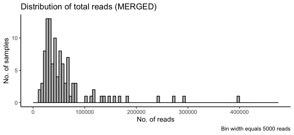
Rarefaction Curves
tmp_select <- ssu_amp_data
tmp_select$metadata$SITE <- factor(tmp_select$metadata$SITE,
                                   levels = c("ALMR", "PAST", "CRIS", "PUCL"))
ssu_rare_curve1 <- amp_rarecurve(
  tmp_select,
  stepsize = 1000,
  color_by = "SITE"
) + scale_colour_manual(values = swel_col)
ssu_rare_curve1 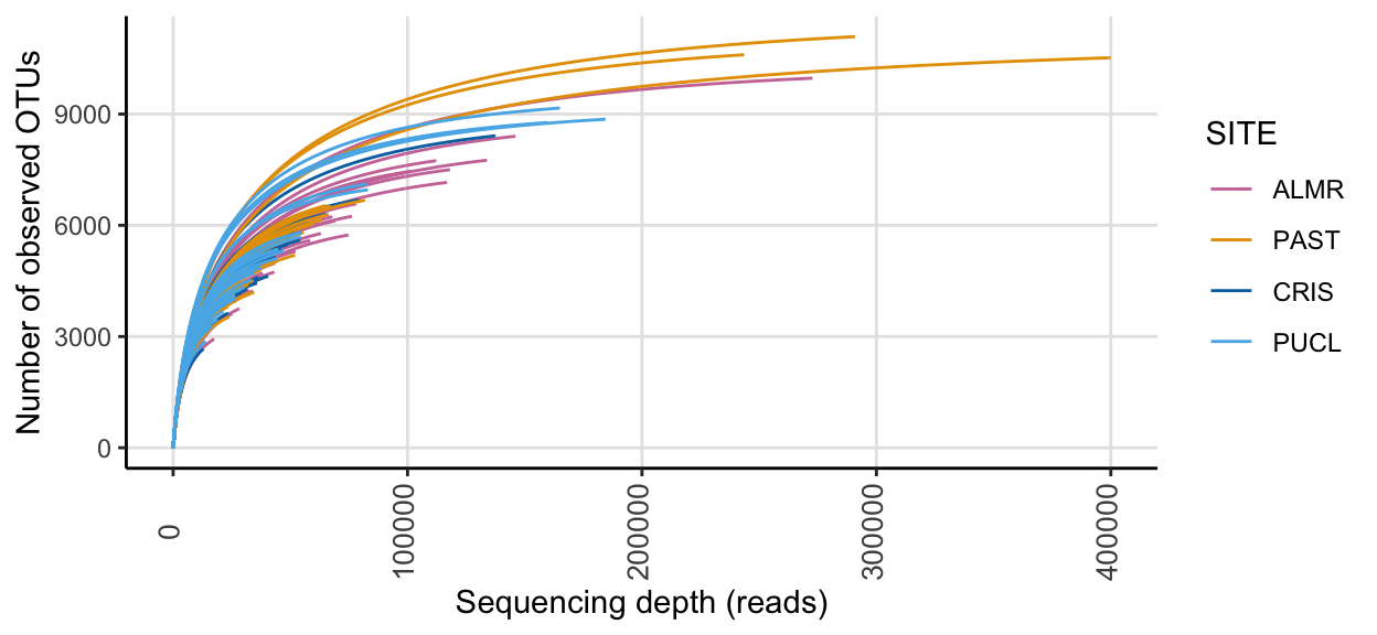
For a quick comparison, we can facet the above data by Site.
ssu_rare_curve2 <- amp_rarecurve(
  tmp_select,
  stepsize = 1000,
  color_by = "SITE",
  facet_by = "SITE",
  facet_scales = "free"
)  + scale_colour_manual(values = swel_col)
ssu_rare_curve2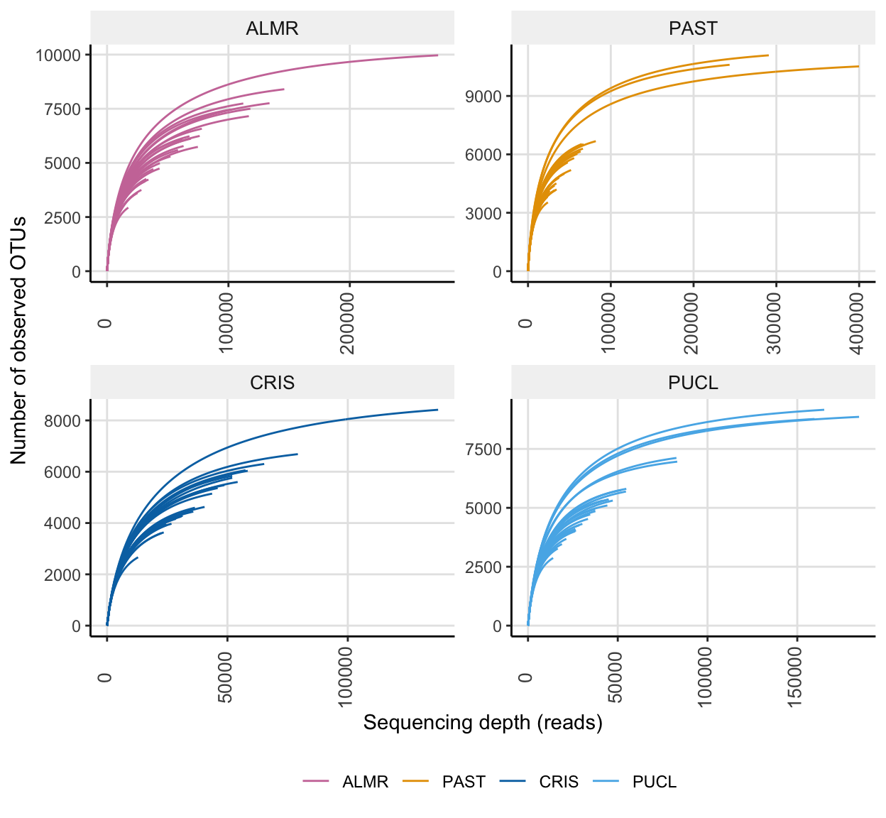
In the full data set, there was a minimum read count of 12882, a median of 44092 reads, and a maximum of 399900 reads. After PIME filtering, there was a minimum read count of 10654, a median of 11922 reads, and a maximum of 12171 reads.
Alpha Diversity
To account for presence of rare sequence variants caused by sequencing errors or other technical artifacts, we use Hill numbers (Alberdi and Gilbert 2019a). Hill numbers allow the weight put on rare versus abundant sequence variants to be scaled while providing intuitive comparisons of diversity levels using “effective number of ASVs” as a measuring unit. This approach allows for balancing the over representation of rare ASVs that might be inflated due to sequencing errors.
We will then use Shapiro-Wilk tests to test for normalcy and then, depending on the results, either use parametric ANOVA or non-parametric Kruskal-Wallis to compare alpha diversity among treatments.
Calculate Hill Numbers
To calculate Hill numbers, we use the R package hilldiv (Alberdi and Gilbert 2019b). We calculate three metrics that put more or less weight on common species:
- Observed richness, where
q-value = 0. - Shannon exponential, which weighs ASVs by their frequency, where
q-value = 1. - Simpson multiplicative inverse, which over weighs abundant ASVs, where
q-value = 2.
We perform each analysis against the full data set and the PIME filtered data set using the function hill_div.
The command is as follows:
hill_div(count = x, qvalue = i, tree = ultrametric_tree), where x is the sample by ASV table, i is the q-value corresponding to the metric of interest and tree is an ultrametric formatted phylogenetic tree (see below).
We first transform all the data to relative abundance values, and compute new trees.
ssu_alpha_ds <- c("ssu_ps_work_merge", "ssu_ps_pime_merge")
objects()
for (i in ssu_alpha_ds) {
tmp_ps <- transform_sample_counts(get(i), function(otu) otu/sum(otu))
tmp_ps@phy_tree <- NULL
tmp_tree <- rtree(ntaxa(tmp_ps), rooted = TRUE,
tip.label = taxa_names(tmp_ps))
tmp_ps_norm <- merge_phyloseq(tmp_ps, sample_data, tmp_tree)
tmp_asv <- data.frame(t(otu_table(tmp_ps_norm)))
tmp_ps_name <- purrr::map_chr(i, ~ paste0(., "_norm"))
assign(tmp_ps_name, tmp_ps_norm)
tmp_asv_name <- purrr::map_chr(i, ~ paste0(., "_tu"))
assign(tmp_asv_name, tmp_asv)
rm(list = ls(pattern = "tmp_"))
}No phylogenetic tree
Next, we run the analysis for all three metrics on the data sets without a tree.
qvalue <- c(0,1,2)
for (i in qvalue) {
  for (j in ssu_alpha_ds) {
     tmp_asv <- get(purrr::map_chr(j, ~ paste0(., "_tu")))
     tmp_df <- data.frame(hill_div(tmp_asv, qvalue = i))
     tmp_df <- tmp_df %>% dplyr::rename("tmp_name" = 1) %>%
                              tibble::rownames_to_column("SamName")
     tmp_name <- purrr::map_chr(j, ~ paste0(., "_h", i))
     print(tmp_name)
     assign(tmp_name, tmp_df)
     rm(list = ls(pattern = "tmp_"))
  }
}
objects(pattern = "_h")
And make summary tables to add back into each ps object.
for (i in ssu_alpha_ds) {
     tmp_obs <- get(purrr::map_chr(i, ~ paste0(., "_h0")))
     tmp_sha <- get(purrr::map_chr(i, ~ paste0(., "_h1")))
     tmp_sim <- get(purrr::map_chr(i, ~ paste0(., "_h2")))
     tmp_hill <- dplyr::left_join(tmp_obs, tmp_sha, by = "SamName") %>%
       dplyr::left_join(., tmp_sim, by = "SamName") %>%
       dplyr::rename("Observed" = 2, "Shannon_exp" = 3, "InvSimpson" = 4)
     tmp_name <- purrr::map_chr(i, ~ paste0(., "_hill"))
     assign(tmp_name, tmp_hill)
     rm(list = ls(pattern = "tmp_"))
}
objects(pattern = "_hill")
And then create the new objects with the diversity data.
With a phylogenetic tree
We can also run the tests using the phylogenetic tree to assess lineage diversity rather that ASV diversity for the PIME data set. For this part we will only use PIME filtered data sets. We do a quick check to ensure the ASV names in the ASV table and the tip names in the new phylogenetic tree are identical.
ssu_alpha_ds_tree <- c("ssu_ps_pime_merge")
qvalue <- c(0,1,2)
for (i in qvalue) {
  for (j in ssu_alpha_ds_tree) {
     tmp_asv <- get(purrr::map_chr(j, ~ paste0(., "_tu")))
     tmp_tree <- get(purrr::map_chr(j, ~ paste0(., "_tree_ult")))
     tmp_df <- data.frame(hill_div(tmp_asv, qvalue = i, tree = tmp_tree))
     tmp_df <- tmp_df %>% dplyr::rename("tmp_name" = 1) %>%
                              tibble::rownames_to_column("SamName")
     tmp_name <- purrr::map_chr(j, ~ paste0(., "_ht", i))
     print(tmp_name)
     assign(tmp_name, tmp_df)
     rm(list = ls(pattern = "tmp_"))
  }
}
objects(pattern="_ht")
save(ssu_ps_pime_ht0, ssu_ps_pime_ht1, ssu_ps_pime_ht2, ssu_ps_pime_merge_ht0,
     ssu_ps_pime_merge_ht1, ssu_ps_pime_merge_ht2,
     file = "files/trepo/alpha/rdata/ssu_ps_pime_hill_tree_tests.rdata")
for (i in ssu_alpha_ds_tree) {
tmp_obs <- get(purrr::map_chr(i, ~ paste0(., "_ht0")))
tmp_sha <- get(purrr::map_chr(i, ~ paste0(., "_ht1")))
tmp_sim <- get(purrr::map_chr(i, ~ paste0(., "_ht2")))
tmp_hill <- dplyr::left_join(tmp_obs, tmp_sha, by = "SamName") %>%
dplyr::left_join(., tmp_sim, by = "SamName") %>%
dplyr::rename("Observed_pt" = 2, "Shannon_exp_pt" = 3, "InvSimpson_pt" = 4)
tmp_name <- purrr::map_chr(i, ~ paste0(., "_hill_t"))
assign(tmp_name, tmp_hill)
rm(list = ls(pattern = "tmp_"))
}
objects()Sample Summary
Now we summarize the data for each sample against all three metrics. The table contains the results of ASV diversity estimates from the full data set and the PIME filtered data set, as well as the lineage diversity from the PIME data set.
The suffix _p indicates metrics for the PIME data set and the suffix _pt indicates the lineage diversity for the PIME data set.
Normality Tests
Before running significance tests, we need to know if data is normally distributed, which will tell use whether to use a parametric or non-parametric test. To test if the data are normally distributed, we use the Shapiro-Wilk Normality test and the Bartlett Test of Homogeneity of Variances.
If the p-values are both not significant (p > 0.05) from the tests, we accept the null hypothesis (that the results are normally distributed) and test for significance between samples using an ANOVA. If the p-values are both significant (p < 0.05), we reject the null hypothesis (that the results are normally distributed) and test for significance between samples using Kruskal-Wallis (non-parametric equivalent of ANOVA).
The commands are as follows:
shapiro.test(x), where x is a numeric vector of alpha diversity values from the sample data table.
bartlett.test(Value ~ Group, data = df) Where Value is the metric of interest, Group in the treatment to compare, and df is the data frame.
First the Shapiro-Wilk Normality test.
ssu_div_tab <- ssu_samp_data_tab
ssu_shap_tests <- c()
for (i in colnames(ssu_div_tab[,7:15])) {
   tmp_name <- purrr::map_chr(i, ~ paste0("ssu_shap_", .))
   ssu_shap_tests <- append(ssu_shap_tests, tmp_name)
   tmp_test <- eval(shapiro.test(ssu_div_tab[[i]]))
   tmp_test$data.name <- tmp_name
   assign(tmp_name, tmp_test)
   rm(list = ls(pattern = "tmp_"))
}
And then the Bartlett Test of Homogeneity of Variances.
ssu_div_tab <- ssu_samp_data_tab
ssu_bart_tests <- c()
for (i in colnames(ssu_div_tab[,7:15])) {
   tmp_name <- purrr::map_chr(i, ~ paste0("ssu_bart_", .))
   ssu_bart_tests <- append(ssu_bart_tests, tmp_name)
   tmp_test <- eval(bartlett.test(ssu_div_tab[[i]] ~ SITE, data = ssu_div_tab))
   tmp_test$data.name <- tmp_name
   assign(tmp_name, tmp_test)
   rm(list = ls(pattern = "tmp_"))
}
Here we see which Shapiro-Wilk Normality and Bartlett tests were significant and which were not for the FULL data set analysis?
for (i in colnames(ssu_div_tab[,7:15])) {
  tmp_get_shap <- get(purrr::map_chr(i, ~ paste0("ssu_shap_", .)))
  tmp_shap_p <- round(tmp_get_shap[[2]], 4)
  tmp_get_bart <- get(purrr::map_chr(i, ~ paste0("ssu_bart_", .)))
  tmp_bart_p <- round(tmp_get_bart[[3]], 4)
  tmp_res <- eval(isTRUE(tmp_get_shap[[2]] > 0.05) & isTRUE(tmp_get_bart[[3]] > 0.05))
  tmp_print <- c(i, "Shapiro p-value =", tmp_shap_p,
                 "Bartlett p-value =", tmp_bart_p,
                 "Are both p-values > 0.05?", tmp_res)
  cat(tmp_print,"\n")
  rm(list = ls(pattern = "tmp_"))
}
Observed Shapiro p-value = 0 Bartlett p-value = 0.0895 Are both p-values > 0.05? FALSE
Observed_p Shapiro p-value = 0.2399 Bartlett p-value = 0.4321 Are both p-values > 0.05? TRUE
Observed_pt Shapiro p-value = 0.2994 Bartlett p-value = 0.4728 Are both p-values > 0.05? TRUE
Shannon_exp Shapiro p-value = 0.0002 Bartlett p-value = 0.1238 Are both p-values > 0.05? FALSE
Shannon_exp_p Shapiro p-value = 0.0024 Bartlett p-value = 0.1272 Are both p-values > 0.05? FALSE
Shannon_exp_pt Shapiro p-value = 0.0065 Bartlett p-value = 0.3507 Are both p-values > 0.05? FALSE
InvSimpson Shapiro p-value = 0.0005 Bartlett p-value = 0.0125 Are both p-values > 0.05? FALSE
InvSimpson_p Shapiro p-value = 0.0002 Bartlett p-value = 0.0531 Are both p-values > 0.05? FALSE
InvSimpson_pt Shapiro p-value = 0 Bartlett p-value = 0.0037 Are both p-values > 0.05? FALSE So wherever the value of both p-values in > 0.05 we can use an ANOVA, otherwise we use Kruskal-Wallis.
Significance Tests
To begin, we need to create a hierarchy variable; a two-column matrix specifying the relationship between samples (first column) and groups (second column).
ssu_hill_hier <- ssu_samp_data_tab
ssu_hill_hier <- ssu_hill_hier %>% dplyr::select("sample_id", "SITE") %>%
  tibble::remove_rownames()
ssu_hill_hier <- ssu_hill_hier[order(ssu_hill_hier$SITE), ]
#ssu_hill_hier$SITE = paste(ssu_hill_hier$SITE, 'C', sep='')
# ADD NEXT LINE TO REORDER BY SITE
#ssu_hill_hier <- ssu_hill_hier[order(factor(ssu_hill_hier$SITE,levels=c(c("ALMR", "PAST", "CRIS", "PUCL")))),]
ssu_hill_hier <- ssu_hill_hier %>% tibble::remove_rownames()
saveRDS(ssu_hill_hier, "files/trepo/alpha/rdata/ssu_merge_hill_hier.rds")
Again, we start by testing significance of ASV diversity for the full data set against each of the three metrics using the div_test function.
The command is as follows:
div_test(countable = x, qvalue = i, hierarchy = hier, tree = ultrametric_tree, posthoc = TRUE), where x is ASV by sample table, i is the q-value corresponding to the metric of interest, hier is the hierarchy matrix, tree is an ultrametric formatted phylogenetic tree (see below), and posthoc indicates whether to run post hoc pairwise analyses.
ssu_alpha_ds_full <- c("ssu_ps_work_merge", "ssu_ps_pime_merge")
qvalue <- c(0,1,2)
for (i in ssu_alpha_ds_full) {
     for (j in qvalue) {
         tmp_get <- get(purrr::map_chr(i, ~ paste0(., "_tu")))
         tmp_test <- div_test(tmp_get, qvalue = j,
                      hierarchy = ssu_hill_hier,
                      posthoc = TRUE)
         tmp_name <- purrr::map_chr(i, ~ paste0(., "_q", j, "_adt"))
         print(tmp_name)
         assign(tmp_name, tmp_test)
         rm(list = ls(pattern = "tmp_"))
 }
}
objects(pattern = "_t")
And then test significance of lineage diversity for the PIME filtered data set only.
ssu_alpha_ds_full_tree <- c("ssu_ps_pime_merge")
qvalue <- c(0,1,2)
for (i in ssu_alpha_ds_full_tree) {
     for (j in qvalue) {
         tmp_get <- get(purrr::map_chr(i, ~ paste0(., "_tu")))
         tmp_tree <- get(purrr::map_chr(i, ~ paste0(., "_tree_ult")))
         tmp_test <- div_test(tmp_get, qvalue = j,
                      hierarchy = ssu_hill_hier,
                      posthoc = TRUE,
                      tree = tmp_tree)
         tmp_name <- purrr::map_chr(i, ~ paste0(., "_t_q", j, "_adt"))
         print(tmp_name)
         assign(tmp_name, tmp_test)
         rm(list = ls(pattern = "tmp_"))
 }
}
save(ssu_ps_pime_merge_t_q0_adt, ssu_ps_pime_merge_t_q1_adt, ssu_ps_pime_merge_t_q2_adt,
file = "files/trepo/alpha/rdata/ssu_ps_pime_merge_hill_lineage_test.rdata")| metric | q-value | normality p-value | homogeneity p-value | method | posthoc method | posthoc p-value |
|---|---|---|---|---|---|---|
| Observed | 0 | 0.0000032 | 0.0894791 | Kruskal-Wallis Test | Dunn test with Benjamini-Hochberg correction | 0.2075816 |
| Shannon exponential | 1 | 0.0001597 | 0.1238040 | Kruskal-Wallis Test | Dunn test with Benjamini-Hochberg correction | 0.0012826 |
| Inverse Simpson | 2 | 0.0005432 | 0.0125484 | Kruskal-Wallis Test | Dunn test with Benjamini-Hochberg correction | 0.0000000 |
Summary of significant tests (ASV diversity).
| metric | q-value | normality p-value | homogeneity p-value | method | posthoc method | posthoc p-value |
|---|---|---|---|---|---|---|
| Observed | 0 | 0.2399448 | 0.4320767 | ANOVA | Tukey post-hoc test | 0.001358 |
| Shannon exponential | 1 | 0.0024114 | 0.1272253 | Kruskal-Wallis Test | Dunn test with Benjamini-Hochberg correction | 0.000000 |
| Inverse Simpson | 2 | 0.0001801 | 0.0530918 | Kruskal-Wallis Test | Dunn test with Benjamini-Hochberg correction | 0.000000 |
Summary of significant tests for PIME filtered data (ASV diversity).
| metric | q-value | normality p-value | homogeneity p-value | method | posthoc method | posthoc p-value |
|---|---|---|---|---|---|---|
| Observed | 0 | 0.2994211 | 0.4728254 | ANOVA | Tukey post-hoc test | 0.0018443 |
| Shannon exponential | 1 | 0.0065482 | 0.3506509 | Kruskal-Wallis Test | Dunn test with Benjamini-Hochberg correction | 0.0000000 |
| Inverse Simpson | 2 | 0.0000001 | 0.0036993 | Kruskal-Wallis Test | Dunn test with Benjamini-Hochberg correction | 0.0000000 |
Summary of significant tests the PIME filtered data (ASV Lineage diversity).
PostHoc Analyses
First let’s check the results of each posthoc analysis.
Detailed results of PostHoc Analyses for each metric
Observed (q-value = 0)
[1] "ASV diversity FULL data set (Observed)"
[1] "Dunn test with Benjamini-Hochberg correction"
                   Z    P.unadj     P.adj
ALMR-CRIS  1.8847836 0.05945906 0.3567544
ALMR-PAST  0.3217923 0.74761003 0.7476100
CRIS-PAST -1.5629913 0.11805465 0.3541640
ALMR-PUCL  1.3055574 0.19170311 0.3834062
CRIS-PUCL -0.5792262 0.56243657 0.6749239
PAST-PUCL  0.9837651 0.32523103 0.4878465
[1] "ASV diversity PIME data set (Observed)"
[1] "Tukey post-hoc test"
diff lwr upr p.adj
CRIS-ALMR -92.00000 -284.733749 100.7337 0.598515244
PAST-ALMR -25.96154 -218.695288 166.7722 0.984958245
PUCL-ALMR 195.19231 2.458558 387.9261 0.045953219
PAST-CRIS 66.03846 -126.695288 258.7722 0.807326224
PUCL-CRIS 287.19231 94.458558 479.9261 0.001012313
PUCL-PAST 221.15385 28.420097 413.8876 0.017745897[1] "Lineage diversity PIME data set (Observed)"
[1] "Tukey post-hoc test"
diff lwr upr p.adj
CRISC-ALMRC -55.29075 -162.066591 51.48509 0.531726143
PASTC-ALMRC -15.22649 -122.002329 91.54935 0.982254750
PUCLC-ALMRC 101.82366 -4.952184 208.59950 0.067369932
PASTC-CRISC 40.06426 -66.711579 146.84010 0.760938419
PUCLC-CRISC 157.11441 50.338566 263.89025 0.001200643
PUCLC-PASTC 117.05014 10.274303 223.82599 0.025809519
[1] "ssu_ps_pime_merge_t_q0_adt"
[2] "ssu_ps_pime_merge_t_q0_adt_plot"
[3] "ssu_ps_pime_t_q0_adt_plot" Shannon exponential (q-value = 1)
[1] "ASV diversity FULL data set(Shannon exponential)"
[1] "Dunn test with Benjamini-Hochberg correction"
                   Z      P.unadj       P.adj
ALMR-CRIS -0.3309864 0.7406547704 0.740654770
ALMR-PAST -1.1584523 0.2466794886 0.370019233
CRIS-PAST -0.8274660 0.4079730079 0.489567610
ALMR-PUCL -3.5856858 0.0003361935 0.002017161
CRIS-PUCL -3.2546994 0.0011351243 0.003405373
PAST-PUCL -2.4272335 0.0152144608 0.030428922
[1] "ASV diversity PIME data set (Shannon exponential)"
[1] "Dunn test with Benjamini-Hochberg correction"
Z P.unadj P.adj
ALMR-CRIS -1.0067503 0.3140548067994535 0.376865768159344
ALMR-PAST -1.2228108 0.2214011623194150 0.332101743479123
CRIS-PAST -0.2160606 0.8289405450268563 0.828940545026856
ALMR-PUCL -6.1922036 0.0000000005932884 0.000000003559731
CRIS-PUCL -5.1854534 0.0000002154900225 0.000000646470067
PAST-PUCL -4.9693928 0.0000006716289164 0.000001343257833[1] "Lineage diversity PIME data set (Shannon exponential)"
[1] "Dunn test with Benjamini-Hochberg correction"
Z P.unadj P.adj
ALMRC-CRISC -0.1287169 0.897581640898052 0.89758164089805
ALMRC-PASTC -0.8872274 0.374956488372791 0.56243473255919
CRISC-PASTC -0.7585105 0.448145451347491 0.53777454161699
ALMRC-PUCLC -5.9347697 0.000000002942582 0.00000001765549
CRISC-PUCLC -5.8060528 0.000000006396279 0.00000001918884
PASTC-PUCLC -5.0475424 0.000000447529571 0.00000089505914Simpson multiplicative (i.e., Inverse Simpson) (q-value = 2)
[1] "ASV diversity FULL data set (Inverse Simpson)"
[1] "Dunn test with Benjamini-Hochberg correction"
                   Z                   P.unadj
ALMR-CRIS -3.5305214 0.00041474141527059112675
ALMR-PAST -3.5856858 0.00033619350474802537016
CRIS-PAST -0.0551644 0.95600749252137762201897
ALMR-PUCL -8.4401528 0.00000000000000003169231
CRIS-PUCL -4.9096314 0.00000091247758276900749
PAST-PUCL -4.8544670 0.00000120710988320547623
                             P.adj
ALMR-CRIS 0.0004976896983247093087
ALMR-PAST 0.0005042902571220380823
CRIS-PAST 0.9560074925213776220190
ALMR-PUCL 0.0000000000000001901539
CRIS-PUCL 0.0000027374327483070224
PAST-PUCL 0.0000024142197664109525
[1] "ASV diversity PIME data set (Inverse Simpson)"
[1] "Dunn test with Benjamini-Hochberg correction"
Z P.unadj
ALMR-CRIS -3.58108879 0.000342165333238837905943
ALMR-PAST -3.55810363 0.000373541947897687608756
CRIS-PAST 0.02298517 0.981662105989184685661542
ALMR-PUCL -8.58266082 0.000000000000000009270339
CRIS-PUCL -5.00157203 0.000000568647142344905631
PAST-PUCL -5.02455719 0.000000504595416401124205
P.adj
ALMR-CRIS 0.00051324799985825683181
ALMR-PAST 0.00044825033747722511967
CRIS-PAST 0.98166210598918468566154
ALMR-PUCL 0.00000000000000005562204
CRIS-PUCL 0.00000113729428468981126
PAST-PUCL 0.00000151378624920337261[1] "Lineage diversity PIME data set (Inverse Simpson)"
[1] "Dunn test with Benjamini-Hochberg correction"
Z P.unadj
ALMRC-CRISC 8.168928 0.0000000000000003111422
ALMRC-PASTC 1.029735 0.3031342249161792512524
CRISC-PASTC -7.139192 0.0000000000009388083534
ALMRC-PUCLC 4.831482 0.0000013552060777679617
CRISC-PUCLC -3.337446 0.0008455213793625449697
PASTC-PUCLC 3.801746 0.0001436797613425384293
P.adj
ALMRC-CRISC 0.000000000000001866853
ALMRC-PASTC 0.303134224916179251252
CRISC-PASTC 0.000000000002816425060
ALMRC-PUCLC 0.000002710412155535923
CRISC-PUCLC 0.001014625655235053834
PASTC-PUCLC 0.000215519642013807630Alpha Diversity Plots
Now we can plot the results from the posthoc analyses for each metric and data set using the function div_test_plot_jjs. I modified the orihginal function (div_test_plot) to control a little of the formatting.
The command is as follows:
div_test_plot(divtest = x, chart = "type", colour = col.pal, posthoc = TRUE, threshold = value)), where x is the results from the div_test function, "type" is chart type (box, jitter, or violin),colour is is a color palette, posthoc indicates whether to run posthoc pairwise analyses, and value is the maximum p-value to show in pairwise posthoc results. WARNING if none of the posthoc results are below the specified threshold, the function will throw an error. Therefore, until this is fixed, all posthoc values are shown.
source("hack_code/div_test_plot_jjs.R")
rm(list=ls(pattern="_adt_plot"))
for (i in objects(pattern="_adt")) {
     tmp_name <- purrr::map_chr(i, ~ paste0(., "_plot"))
     tmp_get <- get(i)
     tmp_get$data <- tmp_get$data[order(factor(tmp_get$data$Group,
                                levels=c(c("ALMR", "PAST", "CRIS", "PUCL")))),]
     tmp_get$data <- tmp_get$data %>% tibble::remove_rownames()
     tmp_df <- div_test_plot_jjs(tmp_get, chart = "box",
                                 colour = swel_col, posthoc = TRUE)
     tmp_df <- ggpar(tmp_df, legend = "none")
     print(tmp_name)
     assign(tmp_name, tmp_df)
     rm(list = ls(pattern = "tmp_"))
}
objects(pattern = "_adt")
Posthoc adjusted p-values given for each pairwise comparison.

Figure 2: Top row = Observed; middle row = Shannon exponential; bottom row = Inverse Simpson. Left = ASV diversity full data set; middle = ASV diversity PIME data set; right = Lineage diversity PIME data set.
Alpha Diversity by Site
Next, we calculate alpha diversity for each site using alpha_div() function, which computes a single alpha diversity value for a group of samples. So we need to create/use data frames containing samples split by group. If a tree object is provided, the computed alpha diversity is based on lineage diversity. We will run the analysis on the FULL and PIME data sets, both with and without trees.
The command is as follows:
alpha_div(countable = x, qvalue = j, tree = ultrametric_tree), where x is a count table , j is the q-value corresponding to the metric of interest, and tree is an ultrametric formatted phylogenetic tree.
Full data set split by site
We will start by splitting the full data set by treatment then generating new trees and ASV tables for each split.
site <- c("ALMR","PAST","CRIS", "PUCL")
for (i in site) {
     tmp_name <- purrr::map_chr(i, ~ paste0("ssu_ps_work_merge_", .))
     tmp_ps <- subset_samples(ssu_ps_work_merge, SITE == i)
     tmp_ps <-  prune_taxa(taxa_sums(tmp_ps) > 0, tmp_ps)
     tmp_ps@phy_tree <- NULL
     tmp_ps_tree <- rtree(ntaxa(tmp_ps), rooted = TRUE,
                            tip.label = taxa_names(tmp_ps))
     tmp_ps <- merge_phyloseq(tmp_ps, sample_data, tmp_ps_tree)
     print(tmp_name)
     assign(tmp_name, tmp_ps)
     tmp_asv <- purrr::map_chr(tmp_name, ~ paste0(., "_tu"))
     tmp_get <- get(tmp_name)
     tmp_get_asv <- t(otu_table(tmp_get))
     print(tmp_asv)
     assign(tmp_asv, tmp_get_asv)
     rm(list = ls(pattern = "tmp_"))
}
As mentioned above, any tree used in the hilldv package must be ultrametric. So we need to convert the trees in order to look at lineage diversity. We will also save copies of each tree since this process takes a while to run.
site <- c("ALMR","PAST","CRIS", "PUCL")
for (i in site) {
     tmp_name <- purrr::map_chr(i, ~ paste0("ssu_ps_work_merge_", .))
     tmp_name_tr <- purrr::map_chr(tmp_name, ~ paste0(., "_tree_ult"))
     tmp_get_name <- get(tmp_name)
     tmp_ult_tree <- force.ultrametric(tmp_get_name@phy_tree, method=c("extend"))
     print(tmp_name_tr)
     assign(tmp_name_tr, tmp_ult_tree)
     save_name <- purrr::map_chr(tmp_name_tr, ~ paste0("files/trepo/alpha/rdata/", ., ".rds"))
     tree <- get(tmp_name_tr)
     saveRDS(tree, save_name)
     rm(list = ls(pattern = "tmp_"))
     rm(save_name)
}
qvalue <- c(0,1,2)
for (i in site) {
for (j in qvalue){
tmp_asv_name <- purrr::map_chr(i, ~ paste0("ssu_ps_work_merge_", ., "_tu"))
tmp_asv_name <- get(tmp_asv_name)
tmp_div_name <- purrr::map_chr(i, ~ paste0("ssu_ps_work_merge_", ., "_aldiv_", j))
print(tmp_div_name)
tmp_alpha_div <- alpha_div(countable = tmp_asv_name, qvalue = j)
assign(tmp_div_name, tmp_alpha_div)
rm(list = ls(pattern = "tmp_"))
}
}qvalue <- c(0,1,2)
for (i in site) {
for (j in qvalue){
tmp_asv_name <- purrr::map_chr(i, ~ paste0("ssu_ps_work_merge_", ., "_tu"))
tmp_asv_name <- get(tmp_asv_name)
tmp_tree_name <- purrr::map_chr(i, ~ paste0("ssu_ps_work_merge_", ., "_tree_ult"))
tmp_tree_name <- get(tmp_tree_name)
tmp_div_name <- purrr::map_chr(i, ~ paste0("ssu_ps_work_merge_", ., "_aldiv_", j, "t"))
print(tmp_div_name)
tmp_alpha_div <- alpha_div(countable = tmp_asv_name, qvalue = j, tree = tmp_tree_name)
assign(tmp_div_name, tmp_alpha_div)
rm(list = ls(pattern = "tmp_"))
}
}PIME filtered data set
For this step, we will use the PIME data set. We start by making new trees and ASV tables for each split.
for (i in site) {
     tmp_name <- purrr::map_chr(i, ~ paste0("ssu_ps_pime_merge_", .))
     tmp_ps <- get(tmp_name)
     tmp_ps@phy_tree <- NULL
     tmp_ps_tree <- rtree(ntaxa(tmp_ps), rooted = TRUE,
                            tip.label = taxa_names(tmp_ps))
     tmp_ps <- merge_phyloseq(tmp_ps, sample_data, tmp_ps_tree)
     print(tmp_name)
     assign(tmp_name, tmp_ps)
     tmp_asv_name <- purrr::map_chr(tmp_name, ~ paste0(., "_tu"))
     tmp_get <- get(tmp_name)
     tmp_asv_tab <- t(otu_table(tmp_get))
     print(tmp_asv_name)
     assign(tmp_asv_name, tmp_asv_tab)
     rm(list = ls(pattern = "tmp_"))
}
for (i in site) {
tmp_name <- purrr::map_chr(i, ~ paste0("ssu_ps_pime_merge_", .))
tmp_tr_name <- purrr::map_chr(tmp_name, ~ paste0(., "_tree_ult"))
tmp_get_name <- get(tmp_name)
ultra_tree <- force.ultrametric(tmp_get_name@phy_tree, method=c("extend"))
print(tmp_tr_name)
assign(tmp_tr_name, ultra_tree)
tmp_save_name <- purrr::map_chr(tmp_tr_name, ~ paste0("files/trepo/alpha/rdata/", ., ".rds"))
tmp_tree <- get(tmp_tr_name)
saveRDS(tmp_tree, tmp_save_name)
rm(list = ls(pattern = "tmp_"))
rm(ultra_tree)
}qvalue <- c(0,1,2)
for (i in site) {
for (j in qvalue){
tmp_asv_name <- purrr::map_chr(i, ~ paste0("ssu_ps_pime_merge_", ., "_tu"))
tmp_asv_name <- get(tmp_asv_name)
tmp_spl_name <- purrr::map_chr(i, ~ paste0("ssu_ps_pime_merge_", ., "_tree_ult"))
tmp_spl_name <- get(tmp_spl_name)
tmp_div_name <- purrr::map_chr(i, ~ paste0("ssu_ps_pime_merge_", ., "_aldiv_", j))
print(tmp_div_name)
tmp_alpha_div <- alpha_div(countable = tmp_asv_name, qvalue = j)
assign(tmp_div_name, tmp_alpha_div)
rm(list = ls(pattern = "tmp_"))
}
}qvalue <- c(0,1,2)
for (i in site) {
for (j in qvalue){
tmp_asv_name <- purrr::map_chr(i, ~ paste0("ssu_ps_pime_merge_", ., "_tu"))
tmp_asv_name <- get(tmp_asv_name)
tmp_spl_name <- purrr::map_chr(i, ~ paste0("ssu_ps_pime_merge_", ., "_tree_ult"))
tmp_spl_name <- get(tmp_spl_name)
tmp_div_name <- purrr::map_chr(i, ~ paste0("ssu_ps_pime_merge_", ., "_aldiv_", j, "t"))
print(tmp_div_name)
tmp_alpha_div <- alpha_div(countable = tmp_asv_name, qvalue = j, tree = tmp_spl_name)
assign(tmp_div_name, tmp_alpha_div)
rm(list = ls(pattern = "tmp_"))
}
}| data set | site | type | Observed (q = 0) | Shannon exponential (q = 1) | Inverse Simpson (q = 2) |
|---|---|---|---|---|---|
| full | ALMR | asv | 5793.808 | 1965.1239 | 564.549518 |
| full | CRIS | asv | 4904.269 | 2021.9701 | 728.151255 |
| full | PAST | asv | 5815.462 | 2128.1377 | 725.065978 |
| full | PUCL | asv | 5292.731 | 2439.9823 | 1067.225431 |
| full | ALMR | lineage | 3203.430 | 305.2822 | 12.429029 |
| full | CRIS | lineage | 2929.589 | 465.2024 | 28.335363 |
| full | PAST | lineage | 3511.358 | 475.1634 | 25.060708 |
| full | PUCL | lineage | 3073.812 | 413.3335 | 13.423236 |
| pime | ALMR | asv | 2839.962 | 1350.6638 | 477.769101 |
| pime | CRIS | asv | 2747.962 | 1410.8571 | 600.482387 |
| pime | PAST | asv | 2814.000 | 1420.8394 | 591.689516 |
| pime | PUCL | asv | 3035.154 | 1736.5943 | 876.520914 |
| pime | ALMR | lineage | 1433.311 | 135.8599 | 5.563441 |
| pime | CRIS | lineage | 1740.892 | 305.8255 | 16.952373 |
| pime | PAST | lineage | 1455.374 | 219.1365 | 15.665769 |
| pime | PUCL | lineage | 1631.922 | 258.5645 | 17.225847 |
Alpha diversity for sample groups from the full and PIME filtered data.
Source Code
The source code for this page can be accessed on GitHub by clicking this link. Please note, that in order to process the data and build the website, we needed to run the workflow and get the results. Then hard code the results and turn off the individual commands. So the raw file for this page is a bit messy—you have been warned.