Hit the Hide Code button to hide the R code.
Synopsis
In order to run the workflow, you either need to first run the DADA2 Workflow and the Data Preparation workflow or begin with the output files from the Data Preparation workflow. See the Data Availability page for complete details.
In this workflow…
Indicator Analysis
- Choose a data set(s) & format data frame(s).
## CODE TO PREFIILTER DATASET
#trim_val <- 100
#for (i in samp_ps) {
#     tmp_get <- get(i)
#     tmp_df <- prune_taxa(taxa_sums(tmp_get) > trim_val, tmp_get)
#     tmp_name <- purrr::map_chr(i, ~ paste0(., "_trim"))
#     assign(tmp_name, tmp_df)
#     rm(list = ls(pattern = "tmp_"))
#}
samp_ps <- c("ssu_ps_work", "ssu_ps_pime", "ssu_ps_work_merge", "ssu_ps_pime_merge")
for (i in samp_ps) {
tmp_get <- get(i)
tmp_df <- data.frame(otu_table(tmp_get))
tmp_df <- tmp_df[, which(colSums(tmp_df) != 0)]
tmp_row_names <- row.names(tmp_df)
tmp_row_names <- tmp_row_names %>%
stringr::str_replace("_W[0-9]{2}_[A-Z]{2}_[A-Z]{2}.*", "")
tmp_df <- tmp_df %>% tibble::add_column(tmp_row_names, .before = 1)
tmp_name <- purrr::map_chr(i, ~ paste0(., "_seq_tab"))
assign(tmp_name, tmp_df)
rm(list = ls(pattern = "tmp_"))
}
objects()- Set the p-value cutoff for the
indvalanalysis.
ssu_p_val <- 0.01- Run Indicator Analysis
set.seed(1191)
for (i in samp_ps) {
     tmp_get <- get(purrr::map_chr(i, ~ paste0(., "_seq_tab")))
     tmp_iva <- indval(tmp_get[,-1], tmp_get[,1])
     tmp_iva_name <- purrr::map_chr(i, ~ paste0(., "_indval_results"))
     #assign(tmp_iva_name, tmp_iva)
     #print(tmp_iva_name)
#################################################################
######### USE THIS CODE BLOCK FOR UNADJUSTED p-VALUES ###########
#################################################################
#     tmp_pv <- tmp_iva$pval[tmp_iva$pval <= ssu_p_val]
#     tmp_gr <- tmp_iva$maxcls[tmp_iva$pval <= ssu_p_val]
#     tmp_iv <- tmp_iva$indcls[tmp_iva$pval <= ssu_p_val]
#     tmp_fr <- apply(tmp_get[,-1] > 0, 2, sum)[tmp_iva$pval <= ssu_p_val]
#     tmp_sum <- data.frame(group = tmp_gr, indval = tmp_iv,
#                                  pval = tmp_pv, freq = tmp_fr)
#################################################################
######### USE THIS CODE BLOCK FOR ADJUSTED p-VALUES #############
#################################################################
     tmp_pv_corrected <- p.adjust(tmp_iva$pval, "fdr")
     tmp_iva$corr_pval <- tmp_pv_corrected
     tmp_iva_name <- purrr::map_chr(i, ~ paste0(., "_indval_results"))
     assign(tmp_iva_name, tmp_iva)
     print(tmp_iva_name)
     tmp_corr_pval <- tmp_iva$pval[tmp_iva$corr_pval <= ssu_p_val]
     tmp_pv <- tmp_iva$pval[tmp_iva$corr_pval <= ssu_p_val]
     tmp_gr <- tmp_iva$maxcls[tmp_iva$corr_pval <= ssu_p_val]
     tmp_iv <- tmp_iva$indcls[tmp_iva$corr_pval <= ssu_p_val]
     tmp_fr <- apply(tmp_get[,-1] > 0, 2, sum)[tmp_iva$corr_pval <= ssu_p_val]
     tmp_sum <- data.frame(group = tmp_gr, indval = tmp_iv, pval = tmp_pv,
                                  corr_pval = tmp_corr_pval, freq = tmp_fr)
#################################################################

     tmp_sum <- tmp_sum[order(tmp_sum$group, -tmp_sum$indval),]

     tmp_tax_df <- data.frame(tax_table(get(i)))
     tmp_tax_df$ASV_ID <- NULL
     tmp_sum_tax <- merge(tmp_sum, tmp_tax_df, by = "row.names", all = TRUE)
     tmp_sum_tax <- tmp_sum_tax[!(is.na(tmp_sum_tax$group)),]
     class(tmp_sum_tax$group) <- "character"
     tmp_sum_tax$group <- stringr::str_replace(tmp_sum_tax$group, "^1$", "ALMR")
     tmp_sum_tax$group <- stringr::str_replace(tmp_sum_tax$group, "^2$", "CRIS")
     tmp_sum_tax$group <- stringr::str_replace(tmp_sum_tax$group, "^3$", "PAST")
     tmp_sum_tax$group <- stringr::str_replace(tmp_sum_tax$group, "^4$", "PUCL")
     tmp_sum_tax <- tmp_sum_tax %>% dplyr::rename("ASV_ID" = "Row.names")
     tmp_sum_tax <- tmp_sum_tax[order(as.numeric(gsub("[A-Z]{3}", "", tmp_sum_tax$ASV_ID))),]
     tmp_sum_tax$ASV_ID <-  as.character(tmp_sum_tax$ASV_ID)
     tmp_res_name <- purrr::map_chr(i, ~ paste0(., "_indval_summary"))
     assign(tmp_res_name, tmp_sum_tax)
     print(tmp_res_name)
     rm(list = ls(pattern = "tmp_"))
}
objects()
Now we save a few files. We first need to reformat the output of the indval function.
for (i in samp_ps) {
     tmp_get <- get(purrr::map_chr(i, ~ paste0(., "_seq_tab")))
     tmp_get[,1] <- NULL
     tmp_df <- as.data.frame(t(tmp_get))
     tmp_col_names <- colnames(tmp_df)
     tmp_col_names <- tmp_col_names %>%
              stringr::str_replace("_W[0-9]{2}_[A-Z]{2}_[A-Z]{2}.*", "")
     colnames(tmp_df) <- tmp_col_names
     #tmp_df$freq_all <- apply(tmp_df > 0, 1, sum)
     tmp_df$freq_ALMR <- apply(tmp_df[ , (names(tmp_df) %in% "ALMR")] > 0, 1, sum)
     tmp_df$freq_CRIS <- apply(tmp_df[ , (names(tmp_df) %in% "CRIS")] > 0, 1, sum)
     tmp_df$freq_PAST <- apply(tmp_df[ , (names(tmp_df) %in% "PAST")] > 0, 1, sum)
     tmp_df$freq_PUCL <- apply(tmp_df[ , (names(tmp_df) %in% "PUCL")] > 0, 1, sum)
     tmp_df$reads_total <- base::rowSums(tmp_df[ , (names(tmp_df) %in% c("ALMR", "CRIS", "PAST", "PUCL"))])
     tmp_df$reads_ALMR <- base::rowSums(tmp_df[ , (names(tmp_df) %in% "ALMR")])
     tmp_df$reads_CRIS <- base::rowSums(tmp_df[ , (names(tmp_df) %in% "CRIS")])
     tmp_df$reads_PAST <- base::rowSums(tmp_df[ , (names(tmp_df) %in% "PAST")])
     tmp_df$reads_PUCL <- base::rowSums(tmp_df[ , (names(tmp_df) %in% "PUCL")])
     tmp_df <- tmp_df[,!grepl("^[ALMR | CRIS | PAST | PUCL]", names(tmp_df))]
     tmp_df <- tmp_df %>% tibble::rownames_to_column("ASV_ID")

     tmp_get_indval <- get(purrr::map_chr(i, ~ paste0(., "_indval_summary")))
     tmp_merge_df <- merge(tmp_df, tmp_get_indval, by = "ASV_ID", all = FALSE)
     tmp_merge_df <- tmp_merge_df[,c(1, 11:14, 2:10, 15:22)]
     tmp_merge_df[order(tmp_merge_df$reads_total, decreasing = TRUE), ]
     tmp_merge_name <- purrr::map_chr(i, ~ paste0(., "_indval_final"))
     assign(tmp_merge_name, tmp_merge_df)
     rm(list = ls(pattern = "tmp_"))
}- Save a new phyloseq object containing only the significant ASVs.
for (i in samp_ps) {
     tmp_get <- get(i)
     tmp_tab <- get(purrr::map_chr(i, ~ paste0(., "_indval_summary")))
     tmp_list <- tmp_tab[,1]
     tmp_ps <- prune_taxa(tmp_list, tmp_get)
     tmp_name <- purrr::map_chr(i, ~ paste0(., "_ind"))
     assign(tmp_name, tmp_ps)
     tmp_ps@phy_tree <- NULL
     tmp_ps <- prune_samples(sample_sums(tmp_ps) > 0, tmp_ps)
     tmp_ps_tree <- rtree(ntaxa(tmp_ps), rooted = TRUE,
                            tip.label = taxa_names(tmp_ps))
     tmp_ps <- merge_phyloseq(tmp_ps, sample_data, tmp_ps_tree)
     assign(tmp_name, tmp_ps)
     rm(list = ls(pattern = "tmp_"))
}
objects(pattern = "_ind")
ssu_ps_pime_merge_ind
Summary of Results
| data set | total reads | indval reads | total ASVs | indval ASVs |
|---|---|---|---|---|
| ALL | 6457054 | 5218639 | 47725 | 10822 |
| ALL-PIME | 711567 | 658224 | 7795 | 7131 |
| MERGE | 6457054 | 4086874 | 47725 | 8494 |
| MERGE-PIME | 1236856 | 1122330 | 11066 | 9575 |
Summary of results from Dufrene-Legendre Indicator Species Analysis (indval) for the ALL & MERGE data sets as well as the corresponding PIME filtered data sets.
FULL Data Set
Remember, the Full data set contains all replicate samples.
All ASVs
First we look at the results of all ASVs.
PIME ASVs
And then the subset of PIME filtered ASVs.
MERGE Data Set
Now we can summarize the merged data set, where replicate samples are collapsed. Again, we look at all ASVs and PIME filtered ASVs.
All ASVs
PIME ASVs
Visualizing DA ASVs/OTUs in Anvi’o
At this point we turn our attention to visualizing the data in anvi’o. We run the same code for all for data sets:
- FULL + all ASVs
- FULL + PIME ASVs
- MERGE + all ASVs
- MERGE + PIME ASVs
We can use the MERGE, PIME filtered data set as an example for what is happening as we move through this portion of the pipeline.
[1] "MERGE, PIME filtered data set"phyloseq-class experiment-level object
otu_table() OTU Table: [ 11066 taxa and 104 samples ]
sample_data() Sample Data: [ 104 samples by 12 sample variables ]
tax_table() Taxonomy Table: [ 11066 taxa by 8 taxonomic ranks ]
phy_tree() Phylogenetic Tree: [ 11066 tips and 11065 internal nodes ]Preparation
Before we start with anvi’o, we need to do a little housekeeping. The first thing we need to do is to change all Proteobacteria classes to phyla, that way we can visualize all of the taxonomy at the phylum level.
- Get all Class-level Proteobacteria names
for (i in samp_ps) {
     tmp_get <- get(i)
     tmp_df <- subset_taxa(tmp_get, Phylum == "Proteobacteria")
     tmp_name <- purrr::map_chr(i, ~paste0(., "_proteo"))
     assign(tmp_name, tmp_df)
     print(tmp_name)
     tmp_get_taxa <- get_taxa_unique(tmp_df,
                                     taxonomic.rank = rank_names(tmp_df)[3],
                                     errorIfNULL=TRUE)
     print(tmp_get_taxa)
     rm(list = ls(pattern = "tmp_"))
     rm(list = ls(pattern = "_proteo"))
}
objects()
"Gammaproteobacteria" "Alphaproteobacteria" "p_Proteobacteria" "Zetaproteobacteria"- Then replace the phylum Proteobacteria with the appropriate class name.
for (j in samp_ps) {
  tmp_name <- purrr::map_chr(j, ~paste0(., "_proteo_clean"))
  tmp_get <- get(j)
  tmp_clean <- data.frame(tax_table(tmp_get))

   for (i in 1:nrow(tmp_clean)){
       if (tmp_clean[i,2] == "Proteobacteria" & tmp_clean[i,3] == "Alphaproteobacteria"){
           phylum <- base::paste("Alphaproteobacteria")
           tmp_clean[i, 2] <- phylum
   }   else if (tmp_clean[i,2] == "Proteobacteria" & tmp_clean[i,3] == "Gammaproteobacteria"){
           phylum <- base::paste("Gammaproteobacteria")
           tmp_clean[i, 2] <- phylum
   }   else if (tmp_clean[i,2] == "Proteobacteria" & tmp_clean[i,3] == "Zetaproteobacteria"){
              phylum <- base::paste("Zetaproteobacteria")
           tmp_clean[i, 2] <- phylum
   }   else if (tmp_clean[i,2] == "Proteobacteria" & tmp_clean[i,3] == "p_Proteobacteria"){
           phylum <- base::paste("p_Proteobacteria")
           tmp_clean[i, 2] <- phylum
       }
     }
  tax_table(tmp_get) <- as.matrix(tmp_clean)
  rank_names(tmp_get)
  assign(tmp_name, tmp_get)
  print(c(tmp_name, tmp_get))
  print(length(get_taxa_unique(tmp_get,
                               taxonomic.rank = rank_names(tmp_get)[2],
                               errorIfNULL=TRUE)))
  tmp_path <- file.path("files/trepo/da/rdata/")
  saveRDS(tmp_get, paste(tmp_path, j, "_clean.rds", sep = ""))
  rm(list = ls(pattern = "tmp_"))
}
rm(class, order, phylum)
objects(pattern="_proteo_clean")
objects()
[1] "MERGE, PIME filtered data set"phyloseq-class experiment-level object
otu_table() OTU Table: [ 11066 taxa and 104 samples ]
sample_data() Sample Data: [ 104 samples by 12 sample variables ]
tax_table() Taxonomy Table: [ 11066 taxa by 8 taxonomic ranks ]
phy_tree() Phylogenetic Tree: [ 11066 tips and 11065 internal nodes ]Anvi’o Workflow
Now we are ready to anvi’o. The goal is to combine the results of the ISA analysis with the distribution of ASVs across each sample. We are going to visualize the data using the anvi’o function anvi-interactive. Anvi’o likes SQLite databases but it also understands that sometimes you don’t have a database. So it offers a manual mode. If you type this command, you can have a look at the pieces of data we need for the visualization, specifically those under the headings MANUAL INPUTS and ADDITIONAL STUFF.
anvi-interactive -hMANUAL INPUTS:
Mandatory input parameters to start the interactive interface without
anvi'o databases.
--manual-mode We need this flag to run anvi'o in an ad hoc
manner, i.e., no database.
-f FASTA, --fasta-file FASTA
A FASTA-formatted input file. This is sort of
optional
-d VIEW_DATA, --view-data VIEW_DATA
A TAB-delimited file for view data. This is the ASV
by sample matrix. We need this
-t NEWICK, --tree NEWICK
NEWICK formatted tree structure. How the ASVs are
ordered in our case.
ADDITIONAL STUFF:
Parameters to provide additional layers, views, or layer data.
-V ADDITIONAL_VIEW, --additional-view ADDITIONAL_VIEW
A TAB-delimited file for an additional view to be used
in the interface. This file should contain all split
names, and values for each of them in all samples.
Each column in this file must correspond to a sample
name. Content of this file will be called 'user_view',
which will be available as a new item in the 'views'
combo box in the interface
-A ADDITIONAL_LAYERS, --additional-layers ADDITIONAL_LAYERS
A TAB-delimited file for additional layer info. In
our case this is info about each ASV. The first column
of the file must be the ASV names, and
the remaining columns should be unique attributes.A few files we generate below cannot be loaded directly. So, in addition to the files that can be loaded when running the interactive, we also have files that must be added to the PROFILE database created by anvi’o when we run the command in --manual-mode.
Here is a nice tutorial on Working with anvi’o additional data tables. A lot of what we need is covered in this tutorial. To get the most out the visualization, we need to create a few files to give anvi’o when we fire up the interactive interface. Additonal details are provided for each step below.
- View data: in our case, a sample by ASV abundance matrix.
- Additional info about each ASV.
- Additional info about each sample.
- Taxa abundance data for each sample at some rank.
- Dendrograms ordering the ASVs and samples (based on view data).
- Fasta file of all ASVs in the analysis.
1. View data
Let’s start with the -d or --view-data file. This file needs to be an ASV by sample matrix of read counts. To simplify the visualization, we will use all ASVs represented by some specified percent of total reads or total read count.
#trim_val <- 100
for (i in samp_ps) {
     tmp_get <- get(purrr::map_chr(i, ~paste0(., "_proteo_clean")))
     tmp_df <- prune_taxa(taxa_sums(tmp_get) > sum(taxa_sums(tmp_get))*0.0005, tmp_get)
     tmp_name <- purrr::map_chr(i, ~ paste0(., "_trim"))
     assign(tmp_name, tmp_df)
     rm(list = ls(pattern = "tmp_"))
}
objects()
[1] "MERGE, PIME filtered data set trimmed by read abundance"phyloseq-class experiment-level object
otu_table() OTU Table: [ 326 taxa and 104 samples ]
sample_data() Sample Data: [ 104 samples by 12 sample variables ]
tax_table() Taxonomy Table: [ 326 taxa by 8 taxonomic ranks ]
phy_tree() Phylogenetic Tree: [ 326 tips and 325 internal nodes ]For this example, before trimming we had 1236856 reads and after trimming we had 462106, a decrease of 774750 reads. Similarly, we had 11066 total ASVs before trimming and 326 ASVs after trimming.
for (i in samp_ps) {
     tmp_get <- get(purrr::map_chr(i, ~ paste0(., "_trim")))
     tmp_df <- as.data.frame(t(otu_table(tmp_get)))
     tmp_df <- tmp_df %>% rownames_to_column("Group")
     tmp_path <- file.path("files/trepo/anvio/")
     write.table(tmp_df, paste(tmp_path, i, "/", "data", ".txt", sep = ""),
            quote = FALSE, sep = "\t", row.names = FALSE)
     rm(list = ls(pattern = "tmp_"))
}
objects()
View data file for MERGE, PIME filtered data set trimmed by read abundance.
   Group ALMR_W01_IB_HS ALMR_W03_IB_HS ALMR_W05_IB_HS ALMR_W07_IB_HS
1 ASV206             14              8             13              6
2  ASV69             17             28             23             13
3 ASV237              5             23              7             16
4  ASV92             27             12             15             16
5  ASV45             24             18             20             29
  ALMR_W09_IB_HS
1              1
2             12
3             14
4              7
5             17
As you can see, the view data is simply an ASV by sample dataframe. Here we display only the first 5 ASVs and 5 samples
We can also transform ASV counts instead.
for (i in samp_ps) {
     tmp_get <- get(purrr::map_chr(i, ~ paste0(., "_trim")))
     tmp_trans <- transform_sample_counts(tmp_get, function(x) 1E5 * {x/sum(x)})
     tmp_df <- as.data.frame(t(otu_table(tmp_trans)))
     tmp_df <- tmp_df %>% rownames_to_column("Group")
     #tmp_name <- purrr::map_chr(i, ~ paste0(., "_trim_tab"))
     #assign(tmp_name, tmp_df)
     tmp_path <- file.path("files/trepo/anvio/")
     write.table(tmp_df, paste(tmp_path, i, "/", "data_", "trans.txt", sep = ""),
            quote = FALSE, sep = "\t", row.names = FALSE)
     rm(list = ls(pattern = "tmp_"))
}
objects()
2. Additional Layers for ASVs
Next, we need some additional data about the ASVs to overlay on the visual. This can be anything, however what we specifically want are the details of the ISA analysis, total reads, and lineage info. I warn you; this code will get ugly and I urge you to find a better way.
for (i in samp_ps) {
     tmp_get_indval <- get(purrr::map_chr(i, ~ paste0(., "_indval_final")))
     tmp_get_indval <- tmp_get_indval %>% dplyr::rename("Group" = "ASV_ID") %>%
                                          dplyr::rename("enriched" = "group")
     tmp_get_indval <- tmp_get_indval[,1:5]
     tmp_get <- get(purrr::map_chr(i, ~ paste0(., "_trim")))
     tmp_otu_df <- as.data.frame(t(otu_table(tmp_get)))
     tmp_total <- cbind(tmp_otu_df, total_reads = rowSums(tmp_otu_df))
     tmp_total <- rev(tmp_total)[1]
     tmp_total <- tmp_total %>% tibble::rownames_to_column("Group")
     tmp_tax_df <- as.data.frame(tax_table(tmp_get))
     tmp_tax_df$ASV_SEQ <- NULL
     tmp_tax_df$ASV_ID <- NULL

     tmp_tax_df <- tmp_tax_df %>% tibble::rownames_to_column("Group")
     tmp_add_lay <- dplyr::left_join(tmp_tax_df, tmp_total, by = "Group") %>%
                   dplyr::left_join(., tmp_get_indval, by = "Group")
     tmp_add_lay$ASV_ID <- tmp_add_lay$Group
     tmp_add_lay <- tmp_add_lay[, c(1,13,8:12,2:7)]
     tmp_path <- file.path("files/trepo/anvio/")
     write.table(tmp_add_lay, paste(tmp_path, i, "/", "additional_layers", ".txt", sep = ""),
            quote = FALSE, sep = "\t", row.names = FALSE, na = "")
     rm(list = ls(pattern = "tmp_"))
}
Here is a small subset of the additional_layers.txt table to demonstrate the format.
| Group | ASV_ID | total_reads | enriched | indval | pval | corr_pval | Kingdom | Phylum | Class | Order | Family | Genus |
|---|---|---|---|---|---|---|---|---|---|---|---|---|
| ASV206 | ASV206 | 709 | PAST | 0.6036671 | 0.001 | 0.001 | Bacteria | Sva0485 | p_Sva0485 | p_Sva0485 | p_Sva0485 | p_Sva0485 |
| ASV69 | ASV69 | 1367 | PAST | 0.3884418 | 0.001 | 0.001 | Bacteria | Acidobacteriota | Aminicenantia | Aminicenantales | o_Aminicenantales | o_Aminicenantales |
| ASV237 | ASV237 | 645 | ALMR | 0.5891473 | 0.001 | 0.001 | Bacteria | Chloroflexi | Anaerolineae | Anaerolineales | Anaerolineaceae | f_Anaerolineaceae |
| ASV92 | ASV92 | 1137 | PAST | 0.5206684 | 0.001 | 0.001 | Bacteria | Desulfobacterota | Desulfobacteria | Desulfatiglandales | Desulfatiglandaceae | Desulfatiglans |
| ASV45 | ASV45 | 1855 | PAST | 0.3757412 | 0.001 | 0.001 | Bacteria | Acidobacteriota | Aminicenantia | Aminicenantales | o_Aminicenantales | o_Aminicenantales |
| ASV345 | ASV345 | 740 | PUCL | 0.6337838 | 0.001 | 0.001 | Bacteria | Nitrospirota | Thermodesulfovibrionia | c_Thermodesulfovibrionia | c_Thermodesulfovibrionia | c_Thermodesulfovibrionia |
| ASV216 | ASV216 | 677 | ALMR | 0.5391433 | 0.001 | 0.001 | Archaea | Asgardarchaeota | Odinarchaeia | c_Odinarchaeia | c_Odinarchaeia | c_Odinarchaeia |
| ASV277 | ASV277 | 693 | NA | NA | NA | Bacteria | Planctomycetota | Phycisphaerae | MSBL9 | SG8-4 | f_SG8-4 | |
| ASV209 | ASV209 | 1086 | CRIS | 0.4972376 | 0.001 | 0.001 | Bacteria | Planctomycetota | Phycisphaerae | Phycisphaerales | Phycisphaeraceae | Urania-1B-19_marine_sediment_group |
| ASV219 | ASV219 | 729 | ALMR | 0.3909465 | 0.001 | 0.001 | Bacteria | Chloroflexi | Dehalococcoidia | GIF9 | AB-539-J10 | SCGC-AB-539-J10 |
3. Additional Views for Samples
Now we want some data about the samples to overlay on the visual. Again, this can be anything. How about a table of alpha diversity metrics? We actually have such a table that was generated way back up the road. Just need to fix the column names.
#metadata_tab <- read.table("files/trepo/dada2/tables/ssu_sample_seq_info.txt", header = TRUE, sep = "\t")
#metadata_tab[,c(2:5)] <- list(NULL)
for (i in samp_ps) {
     tmp_get <- get(i)
     tmp_df <- data.frame(sample_data(tmp_get))
     tmp_df <- tmp_df %>% tibble::rownames_to_column("id")
     tmp_df <- tmp_df %>% dplyr::rename("no_asvs" = "Observed")
     tmp_rc <- data.frame(readcount(tmp_get))
     tmp_rc <- tmp_rc %>% tibble::rownames_to_column("id")
     tmp_rc <- tmp_rc %>% dplyr::rename("no_reads" = 2)
     #identical(tmp_df$id, tmp_rc$id)
     tmp_merge <- dplyr::left_join(tmp_df, tmp_rc)
     tmp_merge <- tmp_merge[, c(1:7,ncol(tmp_merge),8:10)]
     #tmp_final <- dplyr::left_join(tmp_merge, metadata_tab)
     tmp_path <- file.path("files/trepo/anvio/")
     write.table(tmp_merge, paste(tmp_path, i, "/", "additional_views", ".txt", sep = ""),
            quote = FALSE, sep = "\t", row.names = FALSE)
     rm(list = ls(pattern = "tmp_"))
}
Here is a small subset of the additional_views.txt table to demonstrate the format.
| id | SamName | SITE | WEEK | REGION | SEASON | REP | no_reads | no_asvs | Shannon_exp | InvSimpson |
|---|---|---|---|---|---|---|---|---|---|---|
| ALMR_W01_IB_HS | ALMR_W01_IB_HS | ALMR | W01 | IB | HS | R | 12003 | 2879 | 1366.488 | 502.3484 |
| ALMR_W03_IB_HS | ALMR_W03_IB_HS | ALMR | W03 | IB | HS | R | 12137 | 2807 | 1207.189 | 350.6644 |
| ALMR_W05_IB_HS | ALMR_W05_IB_HS | ALMR | W05 | IB | HS | R | 12091 | 2894 | 1356.583 | 437.6661 |
| ALMR_W07_IB_HS | ALMR_W07_IB_HS | ALMR | W07 | IB | HS | R | 11923 | 3122 | 1554.734 | 559.6526 |
| ALMR_W09_IB_HS | ALMR_W09_IB_HS | ALMR | W09 | IB | HS | R | 11893 | 2891 | 1407.963 | 519.2281 |
| ALMR_W11_IB_HS | ALMR_W11_IB_HS | ALMR | W11 | IB | HS | R | 11865 | 2615 | 1247.641 | 457.5817 |
| ALMR_W13_IB_NS | ALMR_W13_IB_NS | ALMR | W13 | IB | NS | R | 12042 | 2831 | 1334.791 | 476.1913 |
| ALMR_W15_IB_NS | ALMR_W15_IB_NS | ALMR | W15 | IB | NS | R | 12082 | 2710 | 1267.159 | 433.6278 |
| ALMR_W17_IB_NS | ALMR_W17_IB_NS | ALMR | W17 | IB | NS | R | 11956 | 3031 | 1444.921 | 528.1189 |
| ALMR_W19_IB_NS | ALMR_W19_IB_NS | ALMR | W19 | IB | NS | R | 12155 | 2485 | 1157.071 | 453.2901 |
4. Taxon rank abundance by sample
The next piece of data is the taxonomic breakdown for each sample. Anvi’o requires a specifically formatted file to display taxonomy. Turned out this was a little tricky to code in R, but thanks to a little nifty block of code written by guoyanzhao on the phyloseq Issues forum, it was a piece of cake. The code can be altered to take any rank. See the post for an explanation.
Anyway, the goal is to sum each taxon at some rank and present that as a bar chart for each sample in the visualization. Anvi’o has a specific format it needs where each row is a sample and each column is a taxon. Taxa names need the prefix t_<RANK>!. For example, t_class! should be added for Class rank.
For the visualizations, we will use the complete data sets, before trimming, so we can capture the total taxonomic composition.
pick_rank <- "Phylum"
pick_rank_l <- "phylum"
for (i in samp_ps) {
# Make the table
    tmp_get <- get(purrr::map_chr(i, ~paste0(., "_proteo_clean")))
    tmp_glom <- tax_glom(tmp_get, taxrank = pick_rank)
    tmp_melt <- psmelt(tmp_glom)
    tmp_melt[[pick_rank]] <- as.character(tmp_melt[[pick_rank]])
    tmp_abund <- aggregate(Abundance ~ Sample + tmp_melt[[pick_rank]], tmp_melt, FUN = sum)
    colnames(tmp_abund)[2] <- "tax_rank"
    tmp_abund <- as.data.frame(cast(tmp_abund, Sample ~ tax_rank))
    tmp_abund <- tibble::remove_rownames(tmp_abund)
    tmp_abund <- tibble::column_to_rownames(tmp_abund, "Sample")
# Reorder table column by sum
    tmp_layers <- tmp_abund[,names(sort(colSums(tmp_abund), decreasing = TRUE))]
# Add the prefix
    tmp_layers <- tmp_layers %>% dplyr::rename_all(function(x) paste0("t_", pick_rank_l,"!", x))
    tmp_layers <- tibble::rownames_to_column (tmp_layers, "taxon")
# save the table
    tmp_path <- file.path("files/trepo/anvio/")
    write.table(tmp_layers, paste(tmp_path, i, "/", "tax_layers", ".txt", sep = ""),
            quote = FALSE, sep = "\t", row.names = FALSE)
    rm(list = ls(pattern = "tmp_"))
}
Here is a small subset of the tax_layers.txt table to demonstrate the format.
| taxon | t_phylum!Alphaproteobacteria | t_phylum!Gammaproteobacteria | t_phylum!Acidobacteriota | t_phylum!Calditrichota | t_phylum!Chloroflexi | t_phylum!Desulfobacterota |
|---|---|---|---|---|---|---|
| ALMR_W01_IB_HS | 112 | 1116 | 1789 | 383 | 1873 | 1077 |
| ALMR_W03_IB_HS | 201 | 1552 | 1351 | 441 | 2257 | 1089 |
| ALMR_W05_IB_HS | 202 | 1403 | 1678 | 494 | 1882 | 1137 |
| ALMR_W07_IB_HS | 176 | 1411 | 1443 | 456 | 1894 | 1174 |
| ALMR_W09_IB_HS | 199 | 1750 | 1332 | 536 | 1955 | 1152 |
| ALMR_W11_IB_HS | 214 | 1860 | 1405 | 603 | 1734 | 1216 |
| ALMR_W13_IB_NS | 191 | 1756 | 1505 | 566 | 1821 | 1135 |
| ALMR_W15_IB_NS | 160 | 1332 | 1533 | 403 | 1929 | 1064 |
| ALMR_W17_IB_NS | 145 | 1073 | 1668 | 477 | 1993 | 1090 |
| ALMR_W19_IB_NS | 151 | 1039 | 1729 | 450 | 1903 | 1177 |
5. Construct Dendrograms
Now we need to generate dendrograms that order the ASVs by their distribution in the samples and the samples by their ASV composition. For this task we will use anvi’o.
The first command reads the view data we generated above and uses Euclidean distance and Ward linkage for hierarchical clustering of the ASVs.
anvi-matrix-to-newick data.txt --distance euclidean \
                               --linkage ward \
                               -o asv.tre
The second command transposes the view data table and then does the same for the samples.
anvi-matrix-to-newick data.txt --distance euclidean \
                               --linkage ward \
                               -o sample.tre \
                               --transpose
There are several distance metrics and linkage methods available. See the help menu for the command by typing anvi-matrix-to-newick -h. Boom.
The ASV tree is fine as is, but the sample tree needs a special format. Specifically, the tree needs to be in a three column, tab delimited, table. This format allows you to add multiple orderings to the same file and view them all in the interactive. The table needs to be in this format:
| item_name | data_type | data_value |
|---|---|---|
| tree_1 | newick | ((P01_D00_010_W8A:0.0250122,P05_D00_010_W8C:0.02,.. |
| tree_2 | newick | ((((((((OTU14195:0.0712585,OTU13230:0.0712585)0:,… |
| (…) | (…) | (…) |
This is easy to do by hand, but I really need the practice, so I will do it in R. Anvi’o is very particular about formatting. For example, the original dendrogram file created by anvi’o ends with a blank line. When we reformt the file, we need to get rid of that blank line or we get an error when trying to import the table.
for (i in samp_ps) {
      tmp_path <- file.path("files/trepo/anvio/")
      tmp_tree <- read_file(paste(tmp_path, i, "/", "sample", ".tre", sep = ""))
      tmp_tree <- gsub("[\r\n]", "", tmp_tree)
      tmp_item <- c("bray_complete")
      tmp_type <- c("newick")
      tmp_df <- c(tmp_tree)
      tmp_tab <- data.frame(tmp_item, tmp_type, tmp_df)
      library(janitor)
      tmp_tab %>% remove_empty("rows")
      colnames(tmp_tab) <- c("item_name",   "data_type",    "data_value")
      write.table(tmp_tab, paste(tmp_path, i, "/", "sample", ".tre", sep = ""),
            sep = "\t", quote = FALSE, row.names = FALSE, na = "")
      rm(list = ls(pattern = "tmp_"))
}
# FOR TRANSFORMED DATA
for (i in samp_ps) {
tmp_path <- file.path("files/trepo/anvio/")
tmp_tree <- read_file(paste(tmp_path, i, "/","sample_", "trans.tre", sep = ""))
tmp_tree <- gsub("[\r\n]", "", tmp_tree)
tmp_item <- c("bray_complete")
tmp_type <- c("newick")
tmp_df <- c(tmp_tree)
tmp_tab <- data.frame(tmp_item, tmp_type, tmp_df)
library(janitor)
tmp_tab %>% remove_empty("rows")
colnames(tmp_tab) <- c("item_name", "data_type", "data_value")
write.table(tmp_tab, paste(tmp_path, i, "/", "sample_", "trans.tre", sep = ""),
sep = "\t", quote = FALSE, row.names = FALSE, na = "")
rm(list = ls(pattern = "tmp_"))
}
objects()6. Make a fasta file
The last piece of data we want is a fasta file of all ASVs in the analysis. We don’t need to add a fasta file, but it is a nice way to keep everything in one place. Plus, you can do BLAST searches directly in the interface by right clicking on the ASV of interest, so it is nice to have the sequences.
for (i in samp_ps) {
       tmp_get <- get(purrr::map_chr(i, ~ paste0(., "_trim")))
       tmp_tab <- tax_table(tmp_get)
       tmp_tab <- tmp_tab[, 7]
       tmp_df <- data.frame(row.names(tmp_tab), tmp_tab)
       colnames(tmp_df) <- c("ASV_ID", "ASV_SEQ")
       tmp_df$ASV_ID <- sub("^", ">", tmp_df$ASV_ID)
       tmp_path <- file.path("files/trepo/anvio/")

       write.table(tmp_df, paste(tmp_path, i, "/", "fasta.fasta", sep = ""),
            sep = "\n", col.names = FALSE, row.names = FALSE,
            quote = FALSE, fileEncoding = "UTF-8")
       rm(list = ls(pattern = "tmp_"))
}
7. Building the Profile Database
Time to put all of these pieces together. This gets a little tricky since we do not yet have a database. Some of the files created above can be loaded directly in the interface while some need to be added to a database. When we fire up the interactive in --manual mode, we must give anvi’o the name of a database and it will create that database for us. Then we can shut down the interactive, add the necessary data files, and start back up.
Here run anvi’o in --manual mode, give it the view-data, tree, and additional-layers files, and a name for the PROFILE data base. Anvi’o will generate the database and populate it with the provided data. It will then open the interactive interface.
anvi-interactive --view-data data.txt \
                 --tree asv.tre \
                 --additional-layers additional_layers.txt \
                 --profile-db profile.db \
                 --manual
If everything looks good, shut down the interactive so we can add more data. So we have a new profile database that we can add the sample metadata (additional_views.txt) and the sample dendrogram (sample.tre) using the command anvi-import-misc-data. This command adds the tables to the new profile.db.
anvi-import-misc-data additional_views.txt \
                      --pan-or-profile-db profile.db \
                      --target-data-table layers
anvi-import-misc-data sample_tree_tab.txt \
                      --pan-or-profile-db profile.db \
                      --target-data-table layer_orders
One last this is to get the table with the taxonomy totals by sample (tax_layers.txt) into the profile database. We will run the same command we just used.
anvi-import-misc-data tax_layers.txt \
                      --pan-or-profile-db profile.db \
                      --target-data-table layers
In fact, we could just as easily append the taxonomy total data onto the additional_layers.txt and import in one command. But we didn’t, so there.
Interactive Interface
With a populated database in hand, we can now begin modifying and exploring the data by running the interactive command again.
anvi-interactive --view-data data.txt \
                 --tree asv.tre \
                 --additional-layers additional_layers.txt \
                 --profile-db profile.db
                 --fasta-file anvio.fasta \
                 --manual
Lineage Maps
#TEMP LOAD ONLY REMOVE WHEN WORKFLOW FINISHED
remove(list = ls())
load("page_build/trepo/da_ssu_wf_2.rdata")
gdata::keep(ssu_ps_pime_merge_trim, sure = TRUE)
load("page_build/trepo/da_ssu_wf_3.rdata")
objects()
[1] "arch_only" "asv_tab1"
[3] "da_samp" "obj"
[5] "ps" "ps_obj"
[7] "ps_water_mc_100" "sam_tab1"
[9] "ssu_pime_merge" "ssu_ps_pime_merge_trim"
[11] "ssu_ps_work_merge" "tax_tab1"
[13] "top_phyl" "total_reads_ps_water"
[15] "total_reads_ps_water_100" "water_mc" ssu_ps_work_merge <- readRDS("files/trepo/data-prep/rdata/ssu_ps_work_merge.rds")
ssu_ps_pime_merge_trim
ssu_pime_merge <- readRDS("files/trepo/pime/rdata/ssu_ps_merge_asv_pime.rds")ps <- ssu_pime_mergeps_water_mc_100 <- prune_taxa(taxa_sums(ps) > 100, ps)
total_reads_ps_water <- sum(readcount(ps))
total_reads_ps_water_100 <- sum(readcount(ps_water_mc_100))
ps_obj <- ps_water_mc_100#summarize_phyloseq(ps_water_o)
#summarize_phyloseq(ps_water_mc)
tax_tab1 <- as.data.frame(tax_table(ps_obj))
tax_tab1 <- tibble::rownames_to_column(tax_tab1, "otu_id")
asv_tab1 <- as.data.frame(t(otu_table(ps_obj)))
asv_tab1 <- tibble::rownames_to_column(asv_tab1, "otu_id")
sam_tab1 <- data.frame(sample_data(ps_obj))
sam_tab1[1] <- NULL
da_samp <- tibble::rownames_to_column(sam_tab1, "sample_id")
water_mc <- merge(asv_tab1, tax_tab1, by="otu_id")
water_mc$ASV_SEQ <- NULLobj <- parse_tax_data(water_mc, class_cols = c("Kingdom", "Phylum",
"Class", "Order",
"Family", "Genus", "ASV_ID" ))
obj$data$tax_abund <- calc_taxon_abund(obj, "tax_data",
cols = da_samp$sample_id)
obj$data$tax_occ <- calc_n_samples(obj, "tax_abund",
groups = da_samp$REGION,
cols = da_samp$sample_id)obj$data$diff_table <- compare_groups(obj,
data = "tax_abund",
cols = da_samp$sample_id,
groups = da_samp$REGION)Bacteria
range.default(obj$data$diff_table$log2_median_ratio, finite=TRUE)[1] -6.483816 6.199672#set.seed(1999)
obj %>%
filter_taxa(taxon_names %in% c("Bacteria"), subtaxa = TRUE) %>%
#filter_taxa(taxon_ranks == "f", supertaxa = TRUE) %>% # subset to the order rank
# filter_taxa(taxon_names %in% c("Proteobacteria", "Bacteroidia", "Archaea"), subtaxa = TRUE, invert = TRUE) # to remove taxa
heat_tree(
node_label = taxon_names,
node_size = n_obs,
# node_size_range = c(0.01, 0.05),
node_label_size_range = c(0.008, 0.04),
node_color = log2_median_ratio,
node_color_interval = c(-6.5, 6.2),
edge_color_interval = c(-6.5, 6.2),
node_color_trans = "area",
node_color_range = c("#0072B2", "gray", "#D55E00"),
node_size_axis_label = "ASV count",
node_color_axis_label = "Log 2 median ratio",
layout = "da",
initial_layout = "re",
overlap_avoidance = 2,
output_file = "files/trepo/da/figures/differential_heat_tree_merged_Bacteria.png")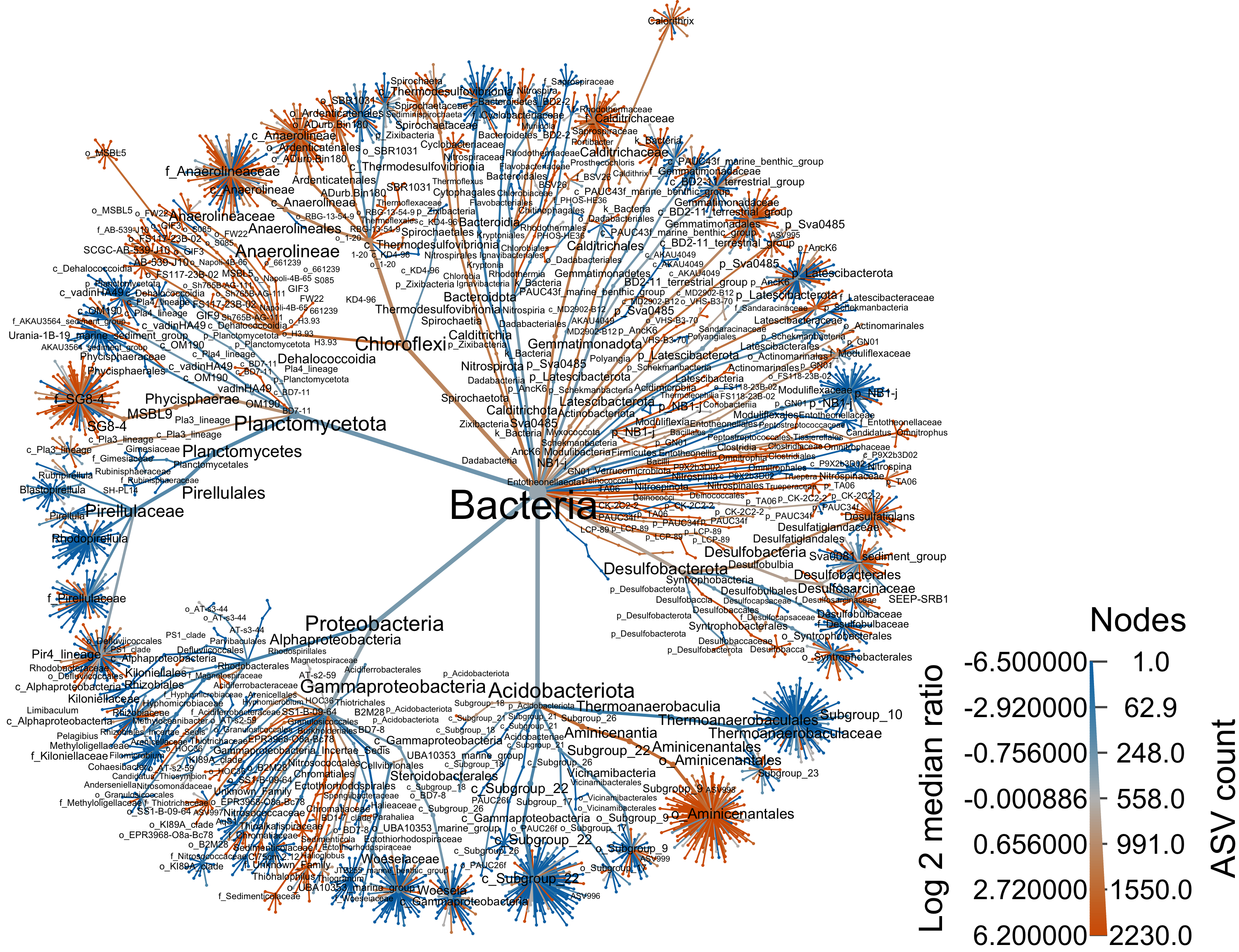
Archaea
arch_only <- obj %>% filter_taxa(taxon_names %in% c("Archaea"), subtaxa = TRUE)
range.default(arch_only$data$diff_table$log2_median_ratio, finite=TRUE)
[1] -6.483816 5.539159#set.seed(1999)
obj %>%
filter_taxa(taxon_names %in% c("Archaea"), subtaxa = TRUE) %>%
# filter_taxa(taxon_ranks == "o", supertaxa = TRUE) %>% # subset to the order rank
# filter_taxa(taxon_names %in% c("Proteobacteria", "Bacteroidia", "Archaea"), subtaxa = TRUE, invert = TRUE) # to remove taxa
heat_tree(
node_label = taxon_names,
node_size = n_obs,
# node_size_range = c(0.01, 0.05),
node_label_size_range = c(0.008, 0.04),
node_color = log2_median_ratio,
node_color_interval = c(-6.5, 5.6),
edge_color_interval = c(-6.5, 5.6),
node_color_trans = "area",
node_color_range = c("#0072B2", "gray", "#D55E00"),
node_size_axis_label = "ASV count",
node_color_axis_label = "Log 2 median ratio",
layout = "ka",
initial_layout = "re",
overlap_avoidance = 2,
output_file = "files/trepo/da/figures/differential_heat_tree_merged_Archaea.png")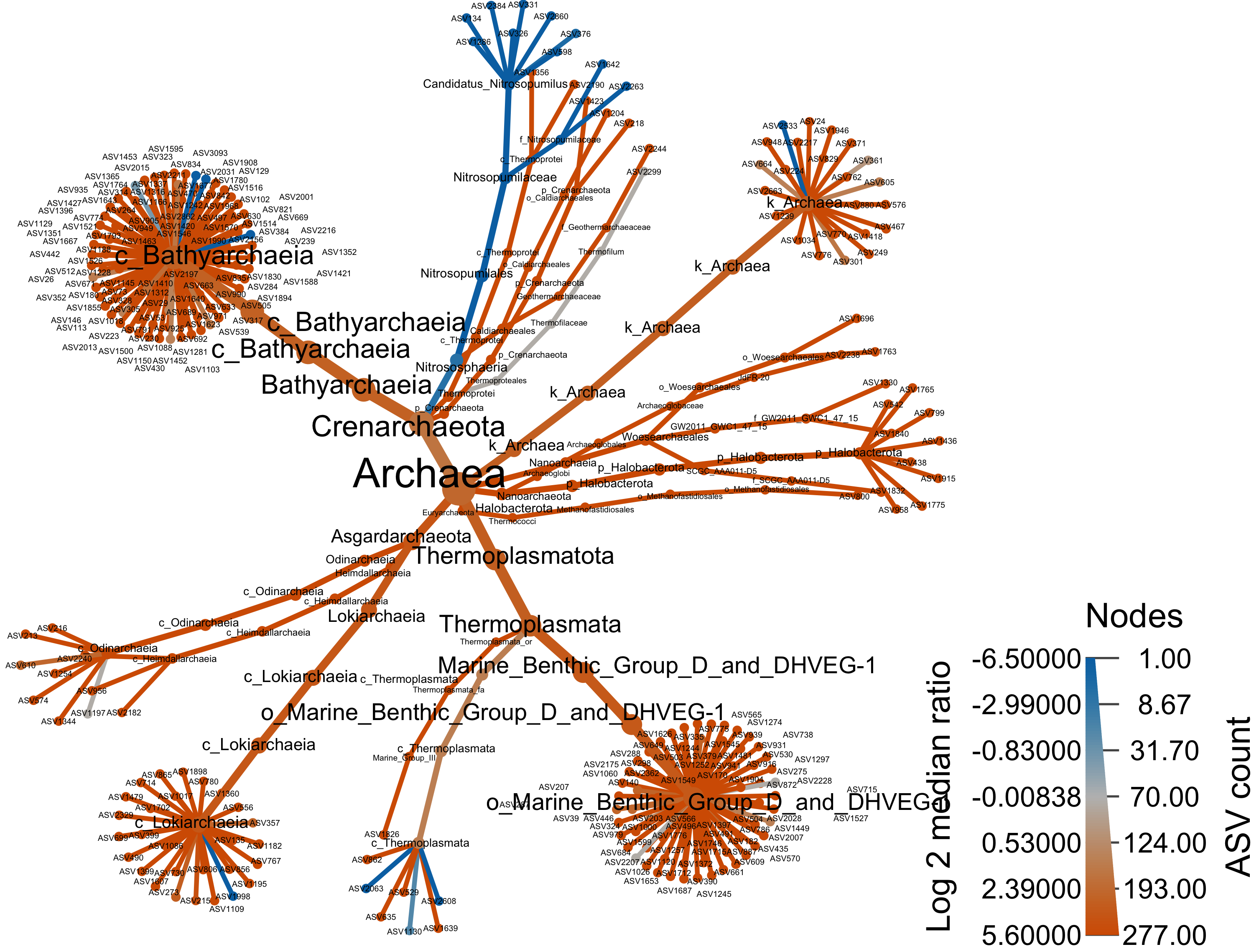
Top Phyla
top_phyl <- obj %>% filter_taxa(taxon_names %in% c("Proteobacteria", "Acidobacteriota", "Chloroflexi", "Planctomycetota"),  subtaxa = TRUE)
range.default(top_phyl$data$diff_table$log2_median_ratio, finite=TRUE)
[1] -5.321928 6.199672#set.seed(10)
obj %>%
filter_taxa(taxon_names %in% c("Proteobacteria", "Acidobacteriota", "Chloroflexi", "Planctomycetota"),
subtaxa = TRUE) %>%
heat_tree(node_label = taxon_names,
node_size = n_obs,
node_color = log2_median_ratio,
node_color_range = c("#0072B2", "gray", "#D55E00"),
node_color_interval = c(-5.3, 6.2),
#edge_color_interval = c(-5.3, 6.2),
#node_color_trans = "area",
tree_label = taxon_names,
layout = "ka",
initial_layout = "re",
node_color_axis_label = "Log 2 median ratio",
node_size_axis_label = "ASV count",
#overlap_avoidance = 2,
output_file = "files/trepo/da/figures/differential_heat_tree_merged_phyla.png")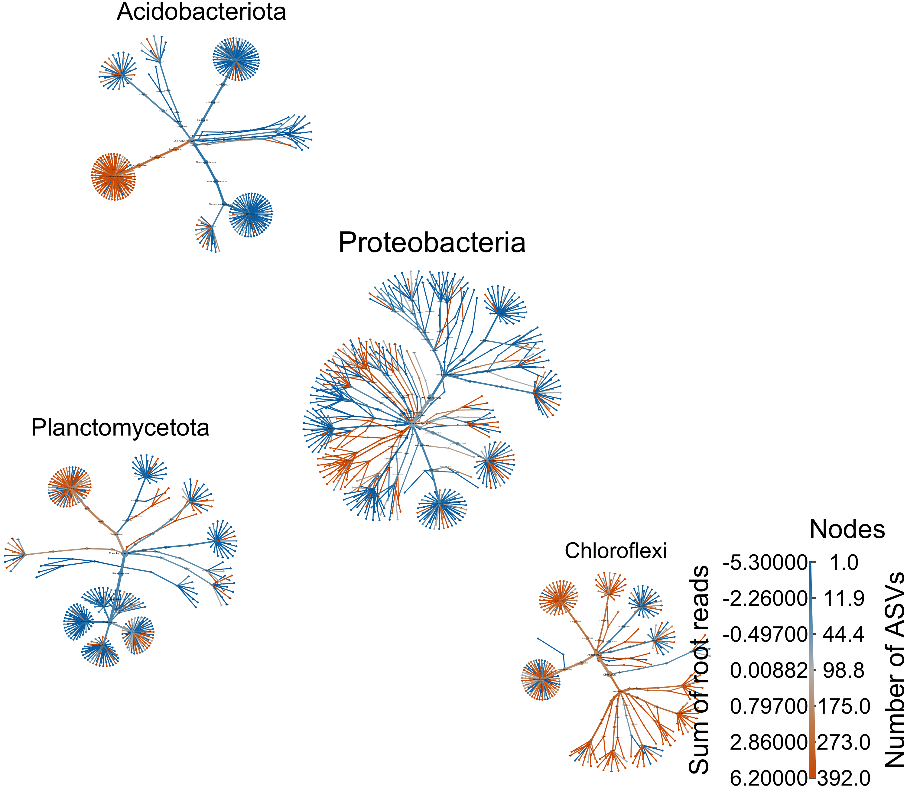
save.image("page_build/trepo/da_ssu_wf_3.rdata")This is code in progress. No peaking
gamma_p <- obj %>% filter_taxa(taxon_names %in% c("Gammaproteobacteria"), subtaxa = TRUE)
range.default(gamma_p$data$diff_table$log2_median_ratio, finite=TRUE)
#set.seed(10)
obj %>%
filter_taxa(taxon_names %in% c("Gammaproteobacteria"),
subtaxa = TRUE) %>%
heat_tree(node_label = taxon_names,
node_size = n_obs,
#node_size_trans = "log10",
node_size_range = c(0.01, 0.05),
edge_size_range = c(0.005, 0.01),
node_label_size_range = c(0.01, 0.04),
node_color = log2_median_ratio,
node_color_range = c("#0072B2", "gray", "#D55E00"),
node_color_interval = c(-5.1, 6.2),
edge_color_interval = c(-5.1, 6.2),
node_color_trans = "area",
tree_label = taxon_names,
layout = "gr",
initial_layout = "re",
node_color_axis_label = "Log 2 median ratio",
node_size_axis_label = "ASV count",
overlap_avoidance = 2,
output_file = "files/trepo/da/figures/differential_heat_tree_merged_gammaprot.png")“automatic,” “reingold-tilford,” “davidson-harel,” “gem,” “graphopt,” “mds,” “fruchterman-reingold,” “kamada-kawai,” “large-graph,” “drl”
obj_site <- parse_tax_data(water_mc, class_cols = c("Kingdom", "Phylum",
                                                    "Class", "Order",
                                                    "Family", "Genus",
                                                    "ASV_ID" ))
obj_site$data$tax_abund <- calc_taxon_abund(obj_site, "tax_data",
                                       cols = da_samp$sample_id)
obj_site$data$tax_occ <- calc_n_samples(obj_site, "tax_abund",
                                   groups = da_samp$SITE,
cols = da_samp$sample_id)obj_site$data$diff_table <- compare_groups(obj_site,
data = "tax_abund",
cols = da_samp$sample_id,
groups = da_samp$SITE,
combinations = list(c('ALMR', 'PAST'),
c('CRIS', 'PUCL')))bact_IB <- obj_site %>% filter_obs("diff_table",
treatment_1 == "ALMR",
treatment_2 == "PAST") %>%
filter_taxa(taxon_names %in% c("Bacteria"), subtaxa = TRUE)
bact_OB <- obj_site %>% filter_obs("diff_table",
treatment_1 == "CRIS",
treatment_2 == "PUCL") %>%
filter_taxa(taxon_names %in% c("Bacteria"), subtaxa = TRUE)
range.default(bact_IB$data$diff_table$log2_median_ratio, finite = TRUE)
range.default(bact_OB$data$diff_table$log2_median_ratio, finite = TRUE)#set.seed(1999)
obj_site %>%
filter_obs("diff_table", treatment_1 == "CRIS", treatment_2 == "PUCL", drop_taxa = TRUE, drop_obs = TRUE) %>%
filter_taxa(taxon_names %in% c("Bacteria"), subtaxa = TRUE) %>%
heat_tree(
node_label = taxon_names,
node_size = n_obs,
# node_size_range = c(0.01, 0.05),
node_label_size_range = c(0.008, 0.04),
node_color = log2_median_ratio,
node_color_interval = c(-3.6, 3.7),
edge_color_interval = c(-3.6, 3.7),
node_color_trans = "area",
node_color_range = c("#009F81", "gray", "#A40122"),
node_size_axis_label = "ASV count",
node_color_axis_label = "Log 2 median ratio",
layout = "da",
initial_layout = "re",
overlap_avoidance = 2,
output_file = "files/trepo/da/figures/differential_heat_tree_merged_Bacteria_OB.png")gamma_p_IB <- obj_site %>% filter_obs("diff_table",
treatment_1 == "ALMR",
treatment_2 == "PAST") %>%
filter_taxa(taxon_names %in% c("Gammaproteobacteria"),
subtaxa = TRUE)
gamma_p_OB <- obj_site %>% filter_obs("diff_table",
treatment_1 == "CRIS",
treatment_2 == "PUCL") %>%
filter_taxa(taxon_names %in% c("Gammaproteobacteria"),
subtaxa = TRUE)
range.default(gamma_p_IB$data$diff_table$log2_median_ratio, finite = TRUE)
range.default(gamma_p_OB$data$diff_table$log2_median_ratio, finite = TRUE)obj_site %>%
filter_obs("diff_table", treatment_1 == "ALMR", treatment_2 == "PAST") %>%
filter_taxa(taxon_names %in% c("Gammaproteobacteria"),
subtaxa = TRUE) %>%
heat_tree(#data = diff_table,
node_label = taxon_names,
node_size = n_obs,
#node_size_trans = "log10",
node_size_range = c(0.01, 0.05),
edge_size_range = c(0.005, 0.01),
node_label_size_range = c(0.01, 0.04),
node_color = log2_median_ratio,
node_color_range = c("#009F81", "gray", "#A40122"),
node_color_interval = c(-5.1, 6.2),
edge_color_interval = c(-5.1, 6.2),
node_color_trans = "area",
tree_label = taxon_names,
layout = "gr",
initial_layout = "re",
node_color_axis_label = "Log 2 median ratio",
node_size_axis_label = "ASV count",
overlap_avoidance = 2,
output_file = "files/trepo/da/figures/differential_heat_tree_merged_gammaprot3.png")Source Code
The source code for this page can be accessed on GitHub by clicking this link. Please note, that in order to process the data and build the website, we needed to run the workflow and get the results. Then hard code the results and turn off the individual commands. So the raw file for this page is a bit messy—you have been warned.