Physical Conditions

Reproducible workflow for … In this workflow, ….

Hit the Hide Code button to hide the R code (shown by default).

Methods

Weekly measurements of physical conditions were collected from October 2017 to March 2020 at four seafloor sites in Almirante Bay. This was done by dangling a YSI Sonde from a boat and collecting measurements approx. 1 m from the seafloor, at 20 ± 5 m (EXO2 & EXO optical DO; Yellow Springs, USA). These sensors were calibrated monthly following the manufacturer’s instructions.

Sites are colored in the below time-series graphs for each parameter. You can highlight a site on the graph by pointing to it with your cursor. Specific values along the timeseries will show up on the top of the graph. You can also zoom into a time period of interest by moving the range selector at the bottom of the graph.

---

Sites
- Almirante: seasonal low oxygen for past 8 years
- Pastores: seasonal low oxygen for past 8 years
- Cristobal: normoxic for past 8 years
- Punta Caracol: normoxic for past 8 years

---

Sensor accuracy and precision:

1. Dissolved Oxygen: accuracy ± 0.1 mg/L
2. Temperature: accuracy ±0.01°C
3. pH: accuracy 0.02 units
4. Chlorophyll: add
5. Cyanobacteria: add

Time-series Analysis

Dissolved Oxygen

First we look at dissolved oxygen values by site over time. Here the function na.locfdeals with any missing data and uses last value to fill gaps. Simple Moving Average (SMA) is a method of time series smoothing and is actually a very basic forecasting technique. It does not need estimation of parameters, but rather is based on order selection. It is a part of smooth package. Here, SMA is a simple moving average that chooses 14 days but 30 days shows clear seasonal signal. At the end of this code block, a raw time-series object with all sites and a smoothed time-series object with all sites are generated.

alm <- ds[which(ds$site == 'Almirante'),]
Alm <- xts(x = alm$DO_mgL, order.by = alm$date)
almir_narm <- na.locf(Alm, fromLast = TRUE)   
Almirante <- SMA(almir_narm, n = 30) 

past <- ds[which(ds$site == 'Pastores'),]
Past <- xts(x = past$DO_mgL, order.by = past$date)
past_narm <- na.locf(Past, fromLast = TRUE)  
Pastores <- SMA(past_narm, n = 30)

pucl <- ds[which(ds$site == 'P_Caracol'),]
P.Cara <- xts(x = pucl$DO_mgL, order.by = pucl$date)
pcara_narm <- na.locf(P.Cara, fromLast = TRUE)  
P.Caracol <- SMA(pcara_narm, n = 30)

cris <- ds[which(ds$site == 'Cristobal'),]
Cris <- xts(x = cris$DO_mgL, order.by = cris$date)
Cris <- na.locf(Cris, fromLast = TRUE)
Cristobal <- SMA(Cris, n = 30)

DO_mgL_raw <- cbind(Alm,Past,P.Cara,Cris)
DO_mgL_smoothed <- cbind(Almirante,Pastores,Cristobal, P.Caracol)

SMOOTHED time-series data

smoothed_do <- dygraph(DO_mgL_smoothed, main = "Dissolved Oxygen (Smoothed)", width = "1000") %>%
  dyHighlight(highlightSeriesOpts = list(strokeWidth = 3)) %>% 
  dyAxis("y", label = "DO mg/L") %>% 
  dyAxis("x", label = "time") %>% 
  dySeries("SMA", label = "Almirante", color = "#CC79A7") %>%
  dySeries("SMA.1", label = "Pastores", color = "#E69F00") %>%
  dySeries("SMA.2", label = "Cristobal", color = "#0072B2") %>%
  dySeries("SMA.3", label = "P.Caracol", color = "#56B4E9") %>%
  dyRangeSelector(dateWindow = dateWindow) %>%
  dyLegend(width = 400)
smoothed_do

RAW time-series data

raw_do <- dygraph(DO_mgL_raw, main = "Dissolved Oxygen (Raw)", width = "1000") %>%
  dyHighlight(highlightSeriesOpts = list(strokeWidth = 3)) %>% 
  dySeries("Alm", label = "Almirante", color = "#CC79A7") %>%
  dySeries("Past", label = "Pastores", color = "#E69F00") %>%
  dySeries("Cris", label = "Cristobal", color = "#0072B2") %>%
  dySeries("P.Cara", label = "P.Caracol", color = "#56B4E9") %>%
  dyRangeSelector(dateWindow = dateWindow) %>%
  dyLegend(width = 400)
raw_do

This is the decomposed dissolved oxygen time series from the Almirante site. Again, na.locf deals with any missing data and uses last value to fill gaps.

Time-series analysis; per site for a specific water parameter

xts_last <- na.locf(Almirante, fromLast = TRUE) 
# plot(xts_last)
# defines time series data as weekly 
xts_ts <- ts(as.numeric(xts_last), frequency = 365.25/7) 
# str(xts_ts) # this should turn it into one column of TS
# calculates all the elements of the TS object, raw, trend, seasonal random
md <- decompose(xts_ts) 
#see decomposed time-series plots
plot(md) 
# mdadj <- xts_ts - md$seasonal # subtract seasonality from TS to reduce noise
# plot(mdadj)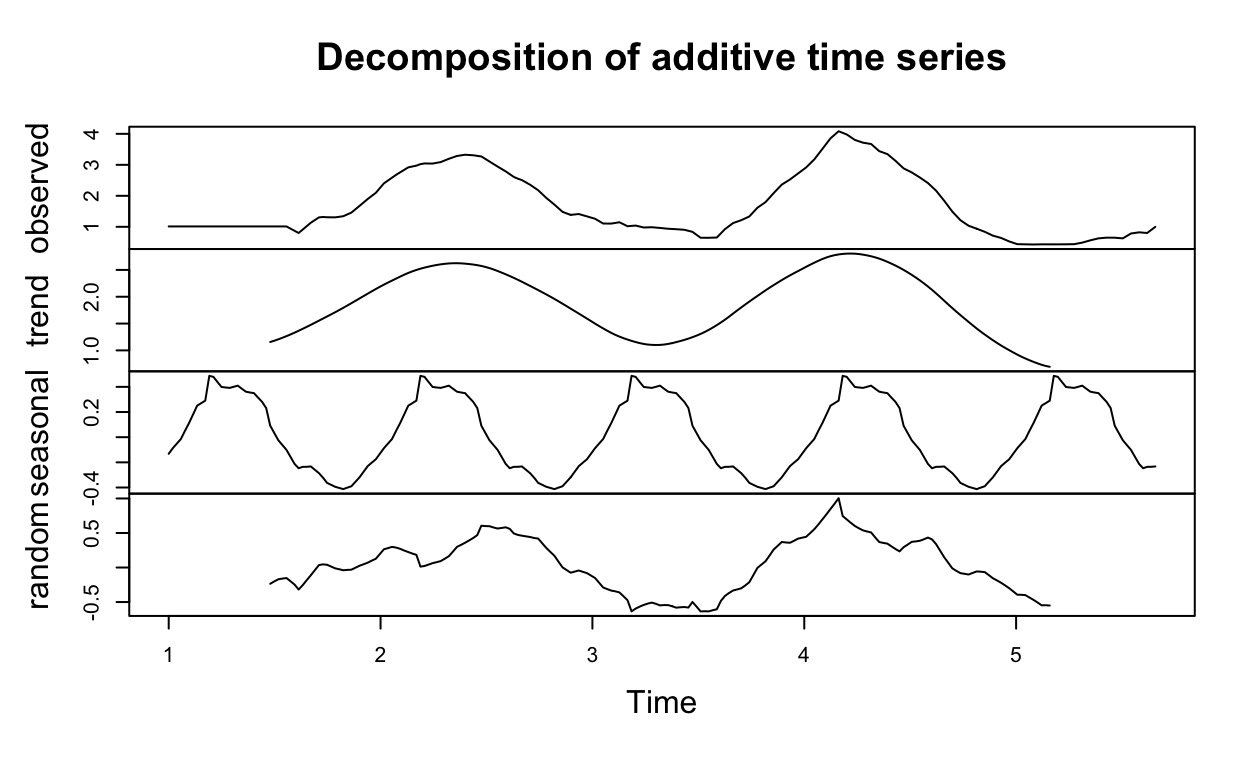 

Temperature

Next, we look at temperature values by site over time. The code here is repeated as above.

alm <- ds[ which(ds$site == 'Almirante'),]
AlmT <- xts(x = alm$temp, order.by = alm$date)
almir_narmT <- na.locf(AlmT, fromLast = TRUE) 
AlmiranteT <- SMA(almir_narmT)

past <- ds[which(ds$site == 'Pastores'),]
PastT <- xts(x = past$temp, order.by = past$date)
past_narmT <- na.locf(PastT, fromLast = TRUE)  
PastoresT <- SMA(past_narmT)

pucl <- ds[which(ds$site == 'P_Caracol'),]
P.CaraT <- xts(x = pucl$temp, order.by = pucl$date)
pcara_narmT <- na.locf(P.CaraT, fromLast = TRUE)  
P.CaracolT <- SMA(pcara_narmT)

cris <- ds[which(ds$site == 'Cristobal'),]
CrisT <- xts(x = cris$temp, order.by = cris$date)
CrisT <- na.locf(CrisT, fromLast= TRUE)
CristobalT <- SMA(CrisT)

temp_raw <- cbind(AlmT,PastT,CrisT,P.CaraT)
temp_smoothed <- cbind(AlmiranteT,PastoresT,CristobalT, P.CaracolT)

SMOOTHED time-series data

smoothed_temp <- dygraph(temp_smoothed, main = "Temperature (Smoothed)", width = "1000") %>%
  dyHighlight(highlightSeriesOpts = list(strokeWidth = 3)) %>% 
  dyAxis("y", label = "Temp. C") %>% 
  dyAxis("x", label = "time") %>% 
  dySeries("SMA", label = "Almirante", color = "#CC79A7") %>%
  dySeries("SMA.1", label = "Pastores", color = "#E69F00") %>%
  dySeries("SMA.2", label = "Cristobal", color = "#0072B2") %>%
  dySeries("SMA.3", label = "P.Caracol", color = "#56B4E9") %>%
  dyRangeSelector(dateWindow = dateWindow) %>%
  dyLegend(width = 400)
smoothed_temp

RAW time-series data

raw_temp <- dygraph(temp_raw, main = "Temperature (Raw)", width = "1000") %>%
  dyHighlight(highlightSeriesOpts = list(strokeWidth = 3)) %>% 
  dySeries("AlmT", label = "Almirante", color = "#CC79A7") %>%
  dySeries("PastT", label = "Pastores", color = "#E69F00") %>%
  dySeries("CrisT", label = "Cristobal", color = "#0072B2") %>%
  dySeries("P.CaraT", label = "P.Caracol", color = "#56B4E9") %>%
  dyRangeSelector(dateWindow = dateWindow) %>%
  dyLegend(width = 400)
raw_temp

Time-series analysis; per site for a specific water parameter

xts_lastT <- na.locf(AlmiranteT, fromLast = TRUE)
# plot(xts_last)
 # defines time series data as weekly 
xts_tsT <- ts(as.numeric(xts_lastT), frequency = 365.25/7)
# str(xts_ts) # this should turn it into one column of TS
 # calculates all the elements of the TS object, raw, trend, seasonal random
mdT <- decompose(xts_tsT)
plot(mdT)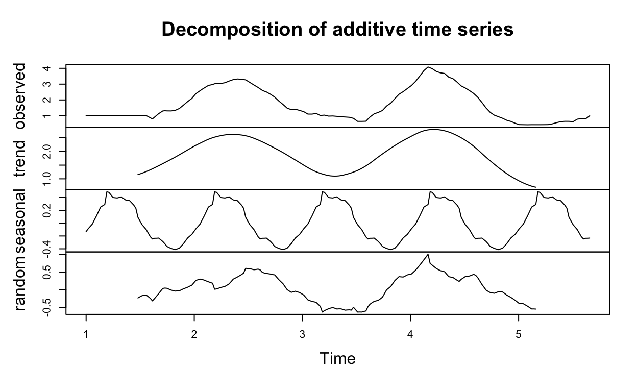

pH

Next, we look at pH values by site over time.

alm <- ds[ which(ds$site == 'Almirante'),]
Alm_pH <- xts(x = alm$pH, order.by = alm$date)
almir_narm_pH <- na.locf(Alm_pH, fromLast= TRUE)
Almirante_pH <- SMA(almir_narm_pH)

past <- ds[which(ds$site == 'Pastores'),]
Past_pH <- xts(x = past$pH, order.by = past$date)
past_narm_pH <- na.locf(Past_pH, fromLast= TRUE)  
Pastores_pH <- SMA(past_narm_pH)

pucl <- ds[which(ds$site == 'P_Caracol'),]
P.Cara_pH <- xts(x = pucl$pH, order.by = pucl$date)
pcara_narm_pH <- na.locf(P.Cara_pH, fromLast= TRUE)  
P.Caracol_pH <- SMA(pcara_narm_pH)

cris <- ds[which(ds$site == 'Cristobal'),]
Cris_pH <- xts(x = cris$pH, order.by = cris$date)
Cris_pH <- na.locf(Cris_pH, fromLast= TRUE)
Cristobal_pH <- SMA(Cris_pH)

pH_raw <- cbind(Alm_pH, Past_pH, Cris_pH, P.Cara_pH)
pH_smoothed <- cbind(Almirante_pH, Pastores_pH, Cristobal_pH, P.Caracol_pH)

SMOOTHED time-series data

smoothed_pH <- dygraph(pH_smoothed, main = "pH (Smoothed)", width = "1000") %>%
  dyHighlight(highlightSeriesOpts = list(strokeWidth = 3))%>% 
  dyAxis("y", label = "pH")%>% 
  dyAxis("x", label = "time")%>% 
  dySeries("SMA", label = "Almirante", color = "#CC79A7") %>%
  dySeries("SMA.1", label = "Pastores", color = "#E69F00") %>%
  dySeries("SMA.2", label = "Cristobal", color = "#0072B2") %>%
  dySeries("SMA.3", label = "P.Caracol", color = "#56B4E9") %>%
  dyRangeSelector(dateWindow = dateWindow) %>%
  dyLegend(width = 400)
smoothed_pH

RAW time-series data

raw_pH <- dygraph(pH_raw, main = "pH (Raw)", width = "1000") %>%
  dyHighlight(highlightSeriesOpts = list(strokeWidth = 3))%>% 
  dySeries("Alm_pH", label = "Almirante", color = "#CC79A7") %>%
  dySeries("Past_pH", label = "Pastores", color = "#E69F00") %>%
  dySeries("Cris_pH", label = "Cristobal", color = "#0072B2") %>%
  dySeries("P.Cara_pH", label = "P.Caracol", color = "#56B4E9") %>%
  dyRangeSelector(dateWindow = dateWindow) %>%
  dyLegend(width = 400)
raw_pH

Time-series analysis; per site for a specific water parameter

xts_last_pH <- na.locf(Alm_pH, fromLast= TRUE)
# plot(xts_last)
xts_ts_pH <- ts(as.numeric(xts_last_pH), frequency = 365.25/7)

md_pH <- decompose(xts_ts_pH)
plot(md_pH)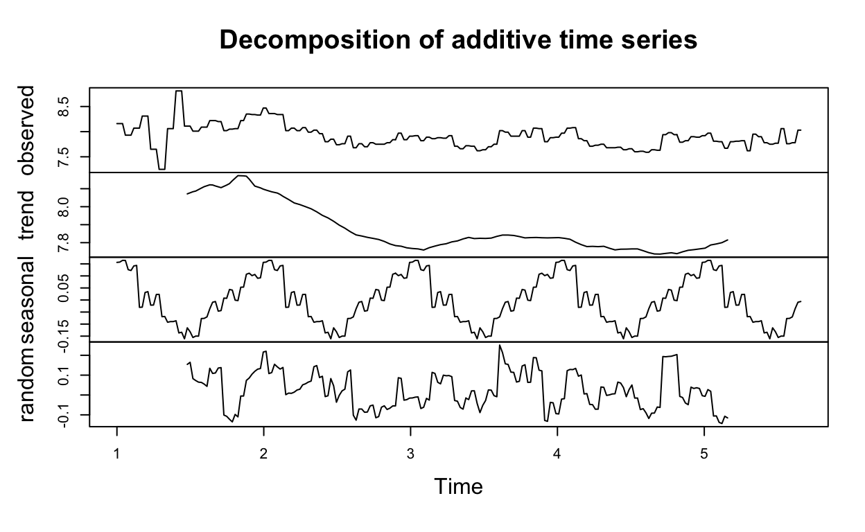

Salinity

Then salinity values by site over time.

alm <- ds[ which(ds$site == 'Almirante'),]
Alm_sal <- xts(x = alm$sal_psu, order.by = alm$date)
almir_narm_sal <- na.locf(Alm_sal, fromLast= TRUE)
Almirante_sal <- SMA(almir_narm_sal)

past <- ds[which(ds$site == 'Pastores'),]
Past_sal <- xts(x = past$sal_psu, order.by = past$date)
past_narm_sal <- na.locf(Past_sal, fromLast= TRUE)  
Pastores_sal <- SMA(past_narm_sal)

pucl <- ds[which(ds$site == 'P_Caracol'),]
P.Cara_sal <- xts(x = pucl$sal_psu, order.by = pucl$date)
pcara_narm_sal <- na.locf(P.Cara_sal, fromLast= TRUE)  
P.Caracol_sal <- SMA(pcara_narm_sal)

cris <- ds[which(ds$site == 'Cristobal'),]
Cris_sal <- xts(x = cris$sal_psu, order.by = cris$date)
Cris_sal <- na.locf(Cris_sal, fromLast= TRUE)
Cristobal_sal <- SMA(Cris_sal)

sal_raw <- cbind(Alm_sal,Past_sal,Cris_sal,P.Cara_sal)
sal_smoothed <- cbind(Almirante_sal,Pastores_sal,Cristobal_sal, P.Caracol_sal)

SMOOTHED time-series data

smoothed_sal <- dygraph(sal_smoothed, main = "Salinity (Smoothed)", width = "1000") %>%
  dyHighlight(highlightSeriesOpts = list(strokeWidth = 3))%>% 
  dyAxis("y", label = "psu")%>% 
  dyAxis("x", label = "time")%>% 
  dySeries("SMA", label = "Almirante", color = "#CC79A7") %>%
  dySeries("SMA.1", label = "Pastores", color = "#E69F00") %>%
  dySeries("SMA.2", label = "Cristobal", color = "#0072B2") %>%
  dySeries("SMA.3", label = "P.Caracol", color = "#56B4E9") %>%
  dyRangeSelector(dateWindow = dateWindow) %>%
  dyLegend(width = 400)
smoothed_sal

RAW time-series data

raw_sal <- dygraph(sal_raw, main = "Salinity (Raw)", width = "1000") %>%
  dyHighlight(highlightSeriesOpts = list(strokeWidth = 3))%>% 
  dySeries("Alm_sal", label = "Almirante", color = "#CC79A7") %>%
  dySeries("Past_sal", label = "Pastores", color = "#E69F00") %>%
  dySeries("Cris_sal", label = "Cristobal", color = "#0072B2") %>%
  dySeries("P.Cara_sal", label = "P.Caracol", color = "#56B4E9") %>%
  dyRangeSelector(dateWindow = dateWindow) %>%
  dyLegend(width = 400)
raw_sal

Time-series analysis; per site for a specific water parameter

xts_last_sal <- na.locf(Alm_sal, fromLast= TRUE)
# plot(xts_last)
xts_ts_sal <- ts(as.numeric(xts_last_sal), frequency = 365.25/7)
# str(xts_ts) # this should turn it into one column of TS
md_sal <- decompose(xts_ts_sal)
plot(md_sal)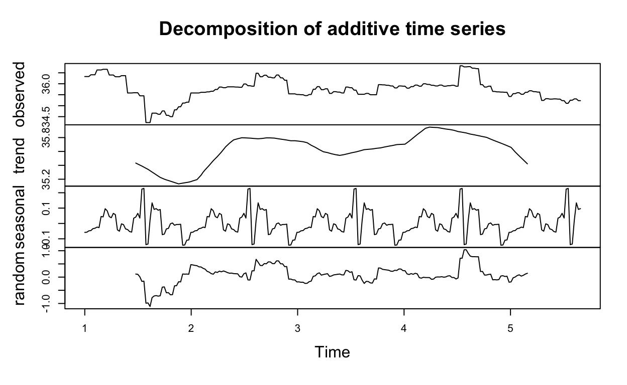

Chlorophyll

Chlorophyll values by site over time.

alm <- ds[ which(ds$site == 'Almirante'),]
Alm_chl <- xts(x = alm$Chlorophyll_ugL, order.by = alm$date)
almir_narm_chl <- na.locf(Alm_chl, fromLast = TRUE)
Almirante_chl <- SMA(almir_narm_chl)

past <- ds[which(ds$site == 'Pastores'),]
Past_chl <- xts(x = past$Chlorophyll_ugL, order.by = past$date)
past_narm_chl <- na.locf(Past_chl, fromLast = TRUE)  
Pastores_chl <- SMA(past_narm_chl)

pucl <- ds[which(ds$site == 'P_Caracol'),]
P.Cara_chl <- xts(x = pucl$Chlorophyll_ugL, order.by = pucl$date)
pcara_narm_chl <- na.locf(P.Cara_chl, fromLast = TRUE)  
P.Caracol_chl <- SMA(pcara_narm_chl)

cris <- ds[which(ds$site == 'Cristobal'),]
Cris_chl <- xts(x = cris$Chlorophyll_ugL, order.by = cris$date)
Cris_chl <- na.locf(Cris_chl, fromLast= TRUE)
Cristobal_chl <- SMA(Cris_chl)

chl_raw <- cbind(Alm_chl,Past_chl,Cris_chl,P.Cara_chl)
chl_smoothed <- cbind(Almirante_chl,Pastores_chl,Cristobal_chl, P.Caracol_chl)

SMOOTHED time-series data

smoothed_chl <- dygraph(chl_smoothed, main = "Chlorophyll (Smoothed)", width = "1000") %>%
  dyHighlight(highlightSeriesOpts = list(strokeWidth = 3)) %>% 
  dyAxis("y", label = "ug/L") %>% 
  dyAxis("x", label = "time") %>% 
  dySeries("SMA", label = "Almirante", color = "#CC79A7") %>%
  dySeries("SMA.1", label = "Pastores", color = "#E69F00") %>%
  dySeries("SMA.2", label = "Cristobal", color = "#0072B2") %>%
  dySeries("SMA.3", label = "P.Caracol", color = "#56B4E9") %>%
  dyRangeSelector(dateWindow = dateWindow) %>%
  dyLegend(width = 400)
smoothed_chl

RAW time-series data

raw_chl <- dygraph(chl_raw, main = "Chlorophyll (Raw)", width = "1000") %>%
  dyHighlight(highlightSeriesOpts = list(strokeWidth = 3)) %>% 
  dySeries("Alm_chl", label = "Almirante", color = "#CC79A7") %>%
  dySeries("Past_chl", label = "Pastores", color = "#E69F00") %>%
  dySeries("Cris_chl", label = "Cristobal", color = "#0072B2") %>%
  dySeries("P.Cara_chl", label = "P.Caracol", color = "#56B4E9") %>%
  dyRangeSelector(dateWindow = dateWindow) %>%
  dyLegend(width = 400)
raw_chl

Time-series analysis; per site for a specific water parameter

xts_last_chl <- na.locf(Alm_chl, fromLast = TRUE)
# plot(xts_last)
xts_ts_chl <- ts(as.numeric(xts_last_chl), frequency = 365.25/7)
# str(xts_ts) 
md_chl <- decompose(xts_ts_chl)
plot(md_chl)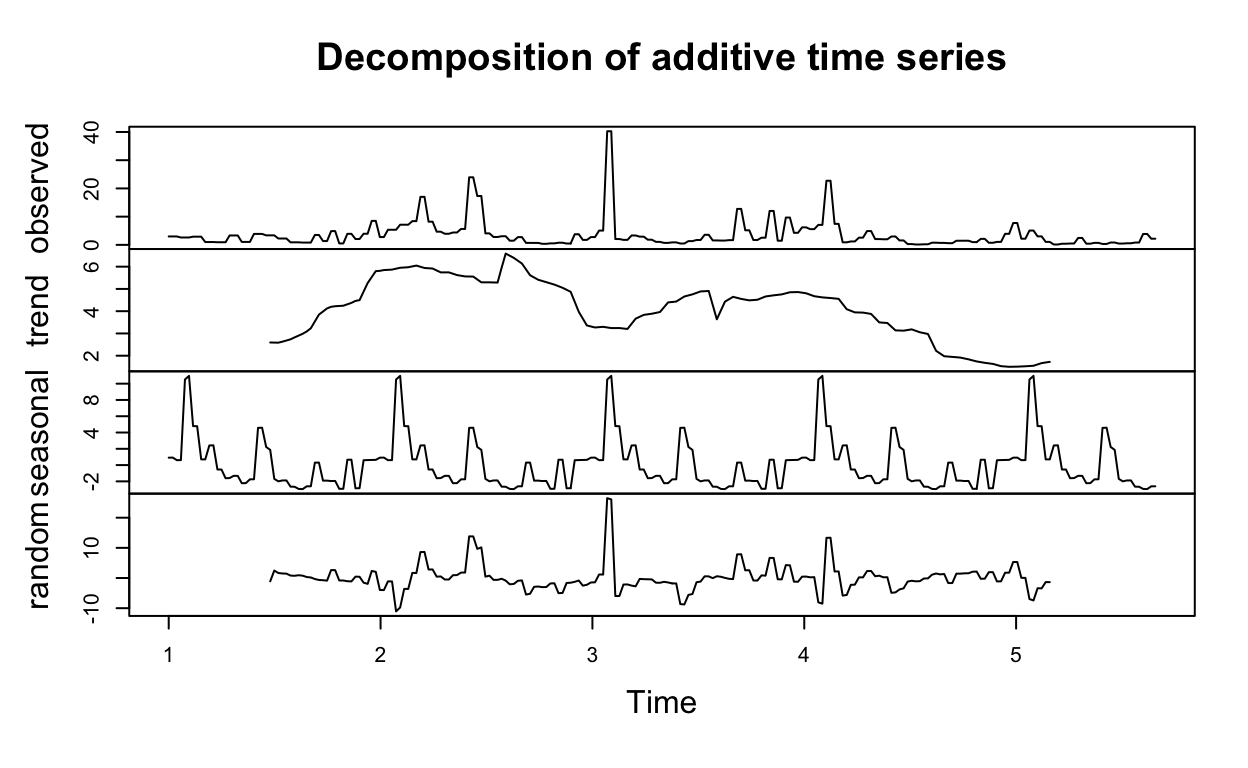 

BGA

And finally, BGA values by site over time.

alm <- ds[ which(ds$site == 'Almirante'),]
Alm_bga <- xts(x = alm$BGA_ugL, order.by = alm$date)
almir_narm_bga <- na.locf(Alm_bga, fromLast = TRUE)
Almirante_bga <- SMA(almir_narm_bga)

past <- ds[which(ds$site == 'Pastores'),]
Past_bga <- xts(x = past$BGA_ugL, order.by = past$date)
past_narm_bga <- na.locf(Past_bga, fromLast = TRUE)  
Pastores_bga <- SMA(past_narm_bga)

pucl <- ds[which(ds$site == 'P_Caracol'),]
P.Cara_bga <- xts(x = pucl$BGA_ugL, order.by = pucl$date)
pcara_narm_bga <- na.locf(P.Cara_bga, fromLast = TRUE)  
P.Caracol_bga <- SMA(pcara_narm_bga)

cris <- ds[which(ds$site == 'Cristobal'),]
Cris_bga <- xts(x = cris$BGA_ugL, order.by = cris$date)
Cris_bga <- na.locf(Cris_bga, fromLast= TRUE)
Cristobal_bga <- SMA(Cris_bga)

bga_raw <- cbind(Alm_bga,Past_bga,Cris_bga,P.Cara_bga)
bga_smoothed <- cbind(Almirante_bga,Pastores_bga,Cristobal_bga, P.Caracol_bga)

SMOOTHED time-series data

smoothed_bga <- dygraph(bga_smoothed, main = "Cyanobacteria (Smoothed)", width = "1000") %>%
  dyHighlight(highlightSeriesOpts = list(strokeWidth = 3)) %>% 
  dyAxis("y", label = "ug/L") %>% 
  dyAxis("x", label = "time") %>% 
  dySeries("SMA", label = "Almirante", color = "#CC79A7") %>%
  dySeries("SMA.1", label = "Pastores", color = "#E69F00") %>%
  dySeries("SMA.2", label = "Cristobal", color = "#0072B2") %>%
  dySeries("SMA.3", label = "P.Caracol", color = "#56B4E9") %>%
  dyRangeSelector(dateWindow = dateWindow) %>%
  dyLegend(width = 400)
smoothed_bga

RAW time-series data

raw_bga <- dygraph(bga_raw, main = "Cyanobacteria (Raw)", width = "1000") %>%
  dyHighlight(highlightSeriesOpts = list(strokeWidth = 3)) %>% 
  dySeries("Alm_bga", label = "Almirante", color = "#CC79A7") %>%
  dySeries("Past_bga", label = "Pastores", color = "#E69F00") %>%
  dySeries("Cris_bga", label = "Cristobal", color = "#0072B2") %>%
  dySeries("P.Cara_bga", label = "P.Caracol", color = "#56B4E9") %>%
  dyRangeSelector(dateWindow = dateWindow) %>%
  dyLegend(width = 400)
raw_bga

Time-series analysis; per site for a specific water parameter

xts_last_bga <- na.locf(Alm_bga, fromLast= TRUE)
# plot(xts_last)
xts_ts_bga <- ts(as.numeric(xts_last_bga), frequency = 365.25/7)
# str(xts_ts) 
md_bga <- decompose(xts_ts_bga)
plot(md_bga)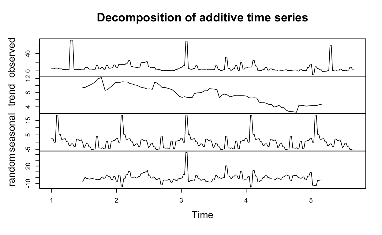

Source Code

The source code for this page can be accessed on GitHub by clicking this link.