Hit the Hide Code button to hide the R code (visible by default).
Summary of Results
In this workflow, we used PIME (Prevalence Interval for Microbiome Evaluation) to filter the FULL 16S rRNA (ASV & OTU) and the MERGED by replicates (ASV & OTU) data sets. The first step in the process is to rarefy the data and then proceed with the filtering. Here is a summary of the results. Tables show comparisons of ASV vs. OTU data sets.
Full Data Set ASV vs. OTU
| Description | no. samples | ASV reads | OTU reads | no. ASVs | no. OTUs |
|---|---|---|---|---|---|
| FULL data set | 304 | 6457054 | 6457054 | 47725 | 21906 |
| Rarefied data | 304 | 820496 | 820496 | 27818 | 13450 |
| PIME filtered data | 304 | 711567 | 740985 | 7795 | 3371 |
| PIME (ALMR) | 76 | 179992 | 186549 | 3417 | 1719 |
| PIME (CRIS) | 76 | 176867 | 184235 | 3336 | 1713 |
| PIME (PAST) | 76 | 175867 | 184770 | 3471 | 1771 |
| PIME (PUCL) | 76 | 178841 | 185431 | 3859 | 1893 |
Merged Data Set ASV vs. OTU
| Description | no. samples | ASV reads | OTU reads | no. ASVs | no. OTUs |
|---|---|---|---|---|---|
| FULL data set | 104 | 6457054 | 6457054 | 47725 | 21910 |
| Rarefied data | 104 | 1339728 | 1339728 | 32423 | 15619 |
| PIME filtered data | 104 | 1236856 | 1269326 | 11066 | 5012 |
| PIME (ALMR) | 26 | 312348 | 319103 | 5222 | 2684 |
| PIME (CRIS) | 26 | 307830 | 316360 | 5136 | 2699 |
| PIME (PAST) | 26 | 306844 | 315960 | 5345 | 2702 |
| PIME (PUCL) | 26 | 309834 | 317903 | 5521 | 2820 |
Prerequisites
This workflow contains diversity assessments for the 16S rRNA data set. In order to run the workflow, you either need to first run the DADA2 Workflow, the Data Preparation workflow, and the OTU clustering workflow. See the Data Availability page for complete details.
Merged Samples (ASV Data)
We will use PIME (Prevalence Interval for Microbiome Evaluation) to create a filtered data set.
Setup
First, choose a phyloseq object and a sample data frame
ssu_pime_ds <- ssu_ps_work_merge
ssu_which_pime <- "ssu_pime_ds"
ssu_pime_ds@phy_tree <- NULL

### USE THIS TO CREATE NEW SAMPLE VARIABLE FOR SPLITTING
##tmp_samp_data <- sample_data(ssu_pime_ds)
#tmp_samp_data$YR_TREAT <- paste(tmp_samp_data$YEAR, tmp_samp_data$TREAT, sep="_")
#tmp_ps <- merge_phyloseq(ssu_pime_ds, tmp_samp_data)
#ssu_pime_ds <- tmp_ps
#rm(list = ls(pattern = "tmp_"))
phyloseq-class experiment-level object
otu_table() OTU Table: [ 47725 taxa and 104 samples ]
sample_data() Sample Data: [ 104 samples by 6 sample variables ]
tax_table() Taxonomy Table: [ 47725 taxa by 8 taxonomic ranks ]And then rarefy the data.
ssu_pime_sample_d <- data.frame(rowSums(otu_table(ssu_pime_ds)))
ssu_pime_sample_d <- ssu_pime_sample_d %>% dplyr::rename(total_reads = 1)

ssu_pime_ds <- rarefy_even_depth(ssu_pime_ds,
                          sample.size = min(ssu_pime_sample_d$total_reads),
                          trimOTUs = TRUE, replace = FALSE, rngseed = 119)
`set.seed(119)` was used to initialize repeatable random subsampling.
Please record this for your records so others can reproduce.
Try `set.seed(119); .Random.seed` for the full vector
15302 OTUs were removed because they are no longer
present in any sample after random subsampling
phyloseq-class experiment-level object
otu_table()   OTU Table:         [ 32423 taxa and 104 samples ]
sample_data() Sample Data:       [ 104 samples by 6 sample variables ]
tax_table()   Taxonomy Table:    [ 32423 taxa by 8 taxonomic ranks ]
The first step in PIME is to define if the microbial community presents a high relative abundance of taxa with low prevalence, which is considered as noise in PIME analysis. This is calculated by random forests analysis and is the baseline noise detection.
ssu_pime.oob.error <- pime.oob.error(ssu_pime_ds, "SITE")[1] 0.01923077Split by Predictor Variable
data.frame(sample_data(ssu_pime_ds))
ssu_per_variable_obj <- pime.split.by.variable(ssu_pime_ds, "SITE")
ssu_per_variable_obj
Detailed results for splitting by sample variables
$ALMR
phyloseq-class experiment-level object
otu_table()   OTU Table:         [ 13892 taxa and 26 samples ]
sample_data() Sample Data:       [ 26 samples by 6 sample variables ]
tax_table()   Taxonomy Table:    [ 13892 taxa by 8 taxonomic ranks ]

$CRIS
phyloseq-class experiment-level object
otu_table()   OTU Table:         [ 15024 taxa and 26 samples ]
sample_data() Sample Data:       [ 26 samples by 6 sample variables ]
tax_table()   Taxonomy Table:    [ 15024 taxa by 8 taxonomic ranks ]

$PAST
phyloseq-class experiment-level object
otu_table()   OTU Table:         [ 15585 taxa and 26 samples ]
sample_data() Sample Data:       [ 26 samples by 6 sample variables ]
tax_table()   Taxonomy Table:    [ 15585 taxa by 8 taxonomic ranks ]

$PUCL
phyloseq-class experiment-level object
otu_table()   OTU Table:         [ 14893 taxa and 26 samples ]
sample_data() Sample Data:       [ 26 samples by 6 sample variables ]
tax_table()   Taxonomy Table:    [ 14893 taxa by 8 taxonomic ranks ]
Calculate Prevalence Intervals
Using the output of pime.split.by.variable, we calculate the prevalence intervals with the function pime.prevalence. This function estimates the highest prevalence possible (no empty ASV table), calculates prevalence for taxa, starting at 5 maximum prevalence possible (no empty ASV table or dropping samples). After prevalence calculation, each prevalence interval are merged.
ssu_prevalences <- pime.prevalence(ssu_per_variable_obj)
ssu_prevalences
Detailed results for all prevalences intervals
$`5`
phyloseq-class experiment-level object
otu_table()   OTU Table:         [ 16911 taxa and 104 samples ]
sample_data() Sample Data:       [ 104 samples by 6 sample variables ]
tax_table()   Taxonomy Table:    [ 16911 taxa by 8 taxonomic ranks ]

$`10`
phyloseq-class experiment-level object
otu_table()   OTU Table:         [ 15028 taxa and 104 samples ]
sample_data() Sample Data:       [ 104 samples by 6 sample variables ]
tax_table()   Taxonomy Table:    [ 15028 taxa by 8 taxonomic ranks ]

$`15`
phyloseq-class experiment-level object
otu_table()   OTU Table:         [ 13479 taxa and 104 samples ]
sample_data() Sample Data:       [ 104 samples by 6 sample variables ]
tax_table()   Taxonomy Table:    [ 13479 taxa by 8 taxonomic ranks ]

$`20`
phyloseq-class experiment-level object
otu_table()   OTU Table:         [ 11066 taxa and 104 samples ]
sample_data() Sample Data:       [ 104 samples by 6 sample variables ]
tax_table()   Taxonomy Table:    [ 11066 taxa by 8 taxonomic ranks ]

$`25`
phyloseq-class experiment-level object
otu_table()   OTU Table:         [ 10039 taxa and 104 samples ]
sample_data() Sample Data:       [ 104 samples by 6 sample variables ]
tax_table()   Taxonomy Table:    [ 10039 taxa by 8 taxonomic ranks ]

$`30`
phyloseq-class experiment-level object
otu_table()   OTU Table:         [ 9145 taxa and 104 samples ]
sample_data() Sample Data:       [ 104 samples by 6 sample variables ]
tax_table()   Taxonomy Table:    [ 9145 taxa by 8 taxonomic ranks ]

$`35`
phyloseq-class experiment-level object
otu_table()   OTU Table:         [ 7668 taxa and 104 samples ]
sample_data() Sample Data:       [ 104 samples by 6 sample variables ]
tax_table()   Taxonomy Table:    [ 7668 taxa by 8 taxonomic ranks ]

$`40`
phyloseq-class experiment-level object
otu_table()   OTU Table:         [ 7052 taxa and 104 samples ]
sample_data() Sample Data:       [ 104 samples by 6 sample variables ]
tax_table()   Taxonomy Table:    [ 7052 taxa by 8 taxonomic ranks ]

$`45`
phyloseq-class experiment-level object
otu_table()   OTU Table:         [ 6479 taxa and 104 samples ]
sample_data() Sample Data:       [ 104 samples by 6 sample variables ]
tax_table()   Taxonomy Table:    [ 6479 taxa by 8 taxonomic ranks ]

$`50`
phyloseq-class experiment-level object
otu_table()   OTU Table:         [ 5411 taxa and 104 samples ]
sample_data() Sample Data:       [ 104 samples by 6 sample variables ]
tax_table()   Taxonomy Table:    [ 5411 taxa by 8 taxonomic ranks ]

$`55`
phyloseq-class experiment-level object
otu_table()   OTU Table:         [ 4934 taxa and 104 samples ]
sample_data() Sample Data:       [ 104 samples by 6 sample variables ]
tax_table()   Taxonomy Table:    [ 4934 taxa by 8 taxonomic ranks ]

$`60`
phyloseq-class experiment-level object
otu_table()   OTU Table:         [ 4495 taxa and 104 samples ]
sample_data() Sample Data:       [ 104 samples by 6 sample variables ]
tax_table()   Taxonomy Table:    [ 4495 taxa by 8 taxonomic ranks ]

$`65`
phyloseq-class experiment-level object
otu_table()   OTU Table:         [ 4089 taxa and 104 samples ]
sample_data() Sample Data:       [ 104 samples by 6 sample variables ]
tax_table()   Taxonomy Table:    [ 4089 taxa by 8 taxonomic ranks ]

$`70`
phyloseq-class experiment-level object
otu_table()   OTU Table:         [ 3312 taxa and 104 samples ]
sample_data() Sample Data:       [ 104 samples by 6 sample variables ]
tax_table()   Taxonomy Table:    [ 3312 taxa by 8 taxonomic ranks ]

$`75`
phyloseq-class experiment-level object
otu_table()   OTU Table:         [ 2987 taxa and 104 samples ]
sample_data() Sample Data:       [ 104 samples by 6 sample variables ]
tax_table()   Taxonomy Table:    [ 2987 taxa by 8 taxonomic ranks ]

$`80`
phyloseq-class experiment-level object
otu_table()   OTU Table:         [ 2672 taxa and 104 samples ]
sample_data() Sample Data:       [ 104 samples by 6 sample variables ]
tax_table()   Taxonomy Table:    [ 2672 taxa by 8 taxonomic ranks ]

$`85`
phyloseq-class experiment-level object
otu_table()   OTU Table:         [ 2021 taxa and 104 samples ]
sample_data() Sample Data:       [ 104 samples by 6 sample variables ]
tax_table()   Taxonomy Table:    [ 2021 taxa by 8 taxonomic ranks ]

$`90`
phyloseq-class experiment-level object
otu_table()   OTU Table:         [ 1693 taxa and 104 samples ]
sample_data() Sample Data:       [ 104 samples by 6 sample variables ]
tax_table()   Taxonomy Table:    [ 1693 taxa by 8 taxonomic ranks ]

$`95`
phyloseq-class experiment-level object
otu_table()   OTU Table:         [ 1354 taxa and 104 samples ]
sample_data() Sample Data:       [ 104 samples by 6 sample variables ]
tax_table()   Taxonomy Table:    [ 1354 taxa by 8 taxonomic ranks ]
Calculate Best Prevalence
Finally, we use the function pime.best.prevalence to calculate the best prevalence. The function uses randomForest to build random forests trees for samples classification and variable importance computation. It performs classifications for each prevalence interval returned by pime.prevalence. Variable importance is calculated, returning the Mean Decrease Accuracy (MDA), Mean Decrease Impurity (MDI), overall and by sample group, and taxonomy for each ASV. PIME keeps the top 30 variables with highest MDA each prevalence level.
set.seed(1911)
ssu_best.prev <- pime.best.prevalence(ssu_prevalences, "SITE")
Interval OOB error rate (%) OTUs Nseqs
1 Prevalence 5% 1.92 16911 1307494
2 Prevalence 10% 0.96 15028 1292012
3 Prevalence 15% 0.96 13479 1274752
4 Prevalence 20% 0 11066 1236856
5 Prevalence 25% 0 10039 1216233
6 Prevalence 30% 0 9145 1195045
7 Prevalence 35% 0 7668 1153904
8 Prevalence 40% 0 7052 1131893
9 Prevalence 45% 0 6479 1109363
10 Prevalence 50% 0 5411 1061161
11 Prevalence 55% 0 4934 1037216
12 Prevalence 60% 0 4495 1012617
13 Prevalence 65% 0 4089 987006
14 Prevalence 70% 0 3312 929687
15 Prevalence 75% 0 2987 898727
16 Prevalence 80% 0 2672 867681
17 Prevalence 85% 0 2021 787247
18 Prevalence 90% 0 1693 738742
19 Prevalence 95% 0 1354 669000ssu_what_is_best <- ssu_best.prev$`OOB error`
ssu_what_is_best[, c(2:4)] <- sapply(ssu_what_is_best[, c(2:4)], as.numeric)
ssu_what_is_best <- ssu_what_is_best %>%
dplyr::rename("OOB_error_rate" = "OOB error rate (%)")
ssu_what_is_best$Interval <- str_replace_all(ssu_what_is_best$Interval, "%", "")
ssu_best <- with(ssu_what_is_best, Interval[which.min(OOB_error_rate)])
ssu_best <- paste("`", ssu_best, "`", sep = "")
ssu_prev_choice <- paste("ssu_best.prev$`Importance`$", ssu_best, sep = "")
ssu_imp_best <- eval(parse(text = (ssu_prev_choice)))Looks like the lowest OOB error rate (%) that retains the most ASVs is 0% from Prevalence 20. We will use this interval.
Best Prevalence Summary
#ssu_imp_best[, 13:14] <- list(NULL)
ssu_imp_best[,(ncol(ssu_imp_best)-1):ncol(ssu_imp_best)] <- list(NULL)
ssu_imp_best <- ssu_imp_best %>% dplyr::rename("ASV_ID" = "SequenceID")
Now we need to create a phyloseq object of ASVs at this cutoff (Prevalence 20).
ssu_best_val <- str_replace_all(ssu_best, "Prevalence ", "")
ssu_best_val <- paste("ssu_prevalences$", ssu_best_val, sep = "")
ssu_prevalence_best <- eval(parse(text = (ssu_best_val)))
saveRDS(ssu_prevalence_best, "rdata/trepo/ssu_merge_asv_prevalence_best.rds")
And look at a summary of the data.
phyloseq-class experiment-level object
otu_table()   OTU Table:         [ 11066 taxa and 104 samples ]
sample_data() Sample Data:       [ 104 samples by 6 sample variables ]
tax_table() Taxonomy Table: [ 11066 taxa by 8 taxonomic ranks ]| Metric | Results |
|---|---|
| Min. number of reads | 10654 |
| Max. number of reads | 12171 |
| Total number of reads | 1236856 |
| Average number of reads | 11893 |
| Mean number of reads | 11893 |
| Median number of reads | 11922 |
| Total ASVS | 11066 |
| Sparsity | 0.742 |
Estimate Error in Prediction
Using the function pime.error.prediction we can estimate the error in prediction. For each prevalence interval, this function randomizes the samples labels into arbitrary groupings using n random permutations, defined by the bootstrap value. For each, randomized and prevalence filtered, data set the OOB error rate is calculated to estimate whether the original differences in groups of samples occur by chance. Results are in a list containing a table and a box plot summarizing the results.
ssu_randomized <- pime.error.prediction(ssu_pime_ds, "TEMP",
                                          bootstrap = 100, parallel = TRUE,
                                          max.prev = 95)
It is also possible to estimate the variation of OOB error for each prevalence interval filtering. This is done by running the random forests classification for n times, determined by the bootstrap value. The function will return a box plot figure and a table for each classification error.
ssu_replicated.oob.error <- pime.oob.replicate(ssu_prevalences, "SITE",
                                               bootstrap = 100, parallel = FALSE)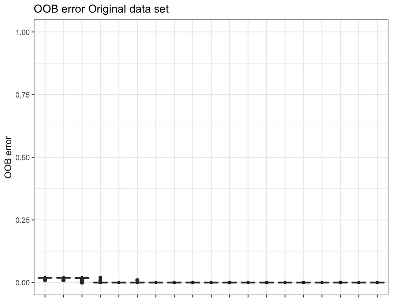
To obtain the confusion matrix from random forests classification use the following:
ssu_prev_confuse <- paste("ssu_best.prev$`Confusion`$", ssu_best, sep = "")
eval(parse(text = (ssu_prev_confuse)))
Save Phyloseq PIME objects
ssu_ps_pime <- ssu_prevalence_best
ssu_ps_pime_tree <- rtree(ntaxa(ssu_ps_pime), rooted = TRUE,
                           tip.label = taxa_names(ssu_ps_pime))
ssu_ps_pime <- merge_phyloseq(ssu_ps_pime,
                               sample_data,
                               ssu_ps_pime_tree)
saveRDS(ssu_ps_pime, "files/trepo/pime/rdata/ssu_ps_merge_asv_pime.rds")
Split & save by predictor variable
ssu_ps_pime_split <- pime.split.by.variable(ssu_ps_pime, "SITE")
saveRDS(ssu_ps_pime_split$ALMR, "files/trepo/pime/rdata/ssu_ps_merge_asv_pime_ALMR.rds")
saveRDS(ssu_ps_pime_split$CRIS, "files/trepo/pime/rdata/ssu_ps_merge_asv_pime_CRIS.rds")
saveRDS(ssu_ps_pime_split$PAST, "files/trepo/pime/rdata/ssu_ps_merge_asv_pime_PAST.rds")
saveRDS(ssu_ps_pime_split$PUCL, "files/trepo/pime/rdata/ssu_ps_merge_asv_pime_PUCL.rds")
$ALMR
phyloseq-class experiment-level object
otu_table() OTU Table: [ 5222 taxa and 26 samples ]
sample_data() Sample Data: [ 26 samples by 6 sample variables ]
tax_table() Taxonomy Table: [ 5222 taxa by 8 taxonomic ranks ]
phy_tree() Phylogenetic Tree: [ 5222 tips and 5221 internal nodes ]
$CRIS
phyloseq-class experiment-level object
otu_table() OTU Table: [ 5136 taxa and 26 samples ]
sample_data() Sample Data: [ 26 samples by 6 sample variables ]
tax_table() Taxonomy Table: [ 5136 taxa by 8 taxonomic ranks ]
phy_tree() Phylogenetic Tree: [ 5136 tips and 5135 internal nodes ]
$PAST
phyloseq-class experiment-level object
otu_table() OTU Table: [ 5345 taxa and 26 samples ]
sample_data() Sample Data: [ 26 samples by 6 sample variables ]
tax_table() Taxonomy Table: [ 5345 taxa by 8 taxonomic ranks ]
phy_tree() Phylogenetic Tree: [ 5345 tips and 5344 internal nodes ]
$PUCL
phyloseq-class experiment-level object
otu_table() OTU Table: [ 5521 taxa and 26 samples ]
sample_data() Sample Data: [ 26 samples by 6 sample variables ]
tax_table() Taxonomy Table: [ 5521 taxa by 8 taxonomic ranks ]
phy_tree() Phylogenetic Tree: [ 5521 tips and 5520 internal nodes ]Create Ampvis2 PIME Object
ssu_otu <- data.frame(t(otu_table(ssu_ps_pime)))
ssu_otu[] <- lapply(ssu_otu, as.numeric)
ssu_otu <- as.matrix(ssu_otu)
ssu_tax <- as.matrix(data.frame(tax_table(ssu_ps_pime)))
ssu_samples <- data.frame(sample_data(ssu_ps_pime))
ssu_ps_amp <- merge_phyloseq(otu_table(ssu_otu, taxa_are_rows = TRUE),
                          tax_table(ssu_tax, ssu_tax),
                          sample_data(ssu_samples))
ssu_amp_asv_pime <- data.frame(otu_table(ssu_ps_amp))
ssu_amp_asv_pime <- ssu_amp_asv_pime %>% tibble::rownames_to_column("OTU")
ssu_amp_tax_pime <- data.frame(tax_table(ssu_ps_amp))
ssu_amp_tax_pime <- ssu_amp_tax_pime %>% tibble::rownames_to_column("OTU")
ssu_amp_tax_pime$ASV_SEQ <- NULL
colnames(ssu_amp_tax_pime)[colnames(ssu_amp_tax_pime) == "ASV_ID"] <- "Species"
ssu_amp_asv_tax_pime <- left_join(ssu_amp_asv_pime, ssu_amp_tax_pime, by = "OTU")
ssu_samp_data_t <- data.frame(ssu_merge_samp_data)
#ssu_samp_data_t[,7:9] <- NULL
ssu_amp_data_pime <- amp_load(ssu_amp_asv_tax_pime, metadata = ssu_samp_data_t)
ssu_diversity_pime <-
amp_alphadiv(
ssu_amp_data_pime,
measure = "observed",
richness = FALSE)
ssu_diversity_pime <-
ssu_diversity_pime %>%
dplyr::rename(
"total_reads" = "Reads",
"total_asvs" = "ObservedOTUs")
ssu_diversity_pime$coverage = cut(ssu_diversity_pime$total_reads,
c(0, 5000, 25000, 100000, 200000),
labels = c(
"low (< 5k)", "medium (5-25k)",
"high (25-100k)", "extra_high (> 100k)"))
ssu_diversity_pime <- ssu_diversity_pime[order(ssu_diversity_pime$SamName), ]
ssu_amp_pime <- amp_load(ssu_amp_asv_tax_pime,
metadata = ssu_diversity_pime, tree = ssu_ps_pime_tree)
ssu_samp_pime <- ssu_diversity_pime
ssu_samp_pime <- ssu_samp_pime %>% tibble::remove_rownames()ampvis2 object with 4 elements.
Summary of OTU table:
Samples OTUs Total#Reads Min#Reads Max#Reads
104 11066 1236856 10654 12171
Median#Reads Avg#Reads
11922 11892.85
Assigned taxonomy:
Kingdom Phylum Class Order Family
11066(100%) 11043(99.79%) 11063(99.97%) 11057(99.92%) 11037(99.74%)
Genus Species
11065(99.99%) 11066(100%)
Metadata variables: 9
SamName, SITE, WEEK, REGION, SEASON, REP, total_reads, total_asvs, coveragesaveRDS(ssu_amp_pime, "files/trepo/pime/rdata/ssu_merge_asv_amp_pime.rds")Summary
Let’s take a look at a table of sample information. Any header with the _p suffix is the PIME filtered data.
And here is how the data sets changed through the PIME filtering process.
| Description | object name | no. samples | total reads | total asvs |
|---|---|---|---|---|
| FULL data set | ssu_ps_work_merge | 104 | 6457054 | 47725 |
| Rarefied data | ssu_pime_ds | 104 | 1339728 | 32423 |
| PIME filtered data | ssu_ps_pime | 104 | 1236856 | 11066 |
| PIME (ALMR) | ssu_ps_pime_ALMR | 26 | 312348 | 5222 |
| PIME (CRIS) | ssu_ps_pime_CRIS | 26 | 307830 | 5136 |
| PIME (PAST) | ssu_ps_pime_PAST | 26 | 306844 | 5345 |
| PIME (PUCL) | ssu_ps_pime_PUCL | 26 | 309834 | 5521 |
Merged Samples (OTU Data)
Setup
First, choose a phyloseq object and a sample data frame
ssu_pime_ds <- ssu_ps_work_merge_otu
ssu_which_pime <- "ssu_pime_ds"
ssu_pime_ds@phy_tree <- NULL

### USE THIS TO CREATE NEW SAMPLE VARIABLE FOR SPLITTING
#tmp_samp_data <- sample_data(ssu_pime_ds)
#tmp_samp_data$YR_TREAT <- paste(tmp_samp_data$YEAR, tmp_samp_data$TREAT, sep="_")
#tmp_ps <- merge_phyloseq(ssu_pime_ds, tmp_samp_data)
#ssu_pime_ds <- tmp_ps
#rm(list = ls(pattern = "tmp_"))
phyloseq-class experiment-level object
otu_table() OTU Table: [ 21910 taxa and 104 samples ]
sample_data() Sample Data: [ 104 samples by 6 sample variables ]
tax_table() Taxonomy Table: [ 21910 taxa by 7 taxonomic ranks ]Then rarefy the data.
ssu_pime_sample_d <- data.frame(rowSums(otu_table(ssu_pime_ds)))
ssu_pime_sample_d <- ssu_pime_sample_d %>% dplyr::rename(total_reads = 1)

ssu_pime_ds <- rarefy_even_depth(ssu_pime_ds,
                                 sample.size = min(ssu_pime_sample_d$total_reads),
                                 trimOTUs = TRUE, replace = FALSE, rngseed = 119)
ssu_pime_ds
`set.seed(119)` was used to initialize repeatable random subsampling.
Please record this for your records so others can reproduce.
Try `set.seed(119); .Random.seed` for the full vector
6291 OTUs were removed because they are no longer
present in any sample after random subsamplingphyloseq-class experiment-level object
otu_table() OTU Table: [ 15619 taxa and 104 samples ]
sample_data() Sample Data: [ 104 samples by 6 sample variables ]
tax_table() Taxonomy Table: [ 15619 taxa by 7 taxonomic ranks ]The first step in PIME is to define if the microbial community presents a high relative abundance of taxa with low prevalence, which is considered as noise in PIME analysis. This is calculated by random forests analysis and is the baseline noise detection.
ssu_pime.oob.error <- pime.oob.error(ssu_pime_ds, "SITE")[1] 0.01923077Split by Predictor Variable
data.frame(sample_data(ssu_pime_ds))
ssu_per_variable_obj <- pime.split.by.variable(ssu_pime_ds, "SITE")
ssu_per_variable_obj
Detailed results for splitting by sample variables
$ALMR
phyloseq-class experiment-level object
otu_table()   OTU Table:         [ 7622 taxa and 26 samples ]
sample_data() Sample Data:       [ 26 samples by 6 sample variables ]
tax_table()   Taxonomy Table:    [ 7622 taxa by 7 taxonomic ranks ]

$CRIS
phyloseq-class experiment-level object
otu_table()   OTU Table:         [ 8030 taxa and 26 samples ]
sample_data() Sample Data:       [ 26 samples by 6 sample variables ]
tax_table()   Taxonomy Table:    [ 8030 taxa by 7 taxonomic ranks ]

$PAST
phyloseq-class experiment-level object
otu_table()   OTU Table:         [ 8314 taxa and 26 samples ]
sample_data() Sample Data:       [ 26 samples by 6 sample variables ]
tax_table()   Taxonomy Table:    [ 8314 taxa by 7 taxonomic ranks ]

$PUCL
phyloseq-class experiment-level object
otu_table()   OTU Table:         [ 7664 taxa and 26 samples ]
sample_data() Sample Data:       [ 26 samples by 6 sample variables ]
tax_table()   Taxonomy Table:    [ 7664 taxa by 7 taxonomic ranks ]
Calculate Prevalence Intervals
Using the output of pime.split.by.variable, we calculate the prevalence intervals with the function pime.prevalence. This function estimates the highest prevalence possible (no empty ASV table), calculates prevalence for taxa, starting at 5 maximum prevalence possible (no empty ASV table or dropping samples). After prevalence calculation, each prevalence interval are merged.
ssu_prevalences <- pime.prevalence(ssu_per_variable_obj)
ssu_prevalences
Detailed results for all prevalences intervals
$`5`
phyloseq-class experiment-level object
otu_table()   OTU Table:         [ 8646 taxa and 104 samples ]
sample_data() Sample Data:       [ 104 samples by 6 sample variables ]
tax_table()   Taxonomy Table:    [ 8646 taxa by 7 taxonomic ranks ]

$`10`
phyloseq-class experiment-level object
otu_table()   OTU Table:         [ 7612 taxa and 104 samples ]
sample_data() Sample Data:       [ 104 samples by 6 sample variables ]
tax_table()   Taxonomy Table:    [ 7612 taxa by 7 taxonomic ranks ]

$`15`
phyloseq-class experiment-level object
otu_table()   OTU Table:         [ 6907 taxa and 104 samples ]
sample_data() Sample Data:       [ 104 samples by 6 sample variables ]
tax_table()   Taxonomy Table:    [ 6907 taxa by 7 taxonomic ranks ]

$`20`
phyloseq-class experiment-level object
otu_table()   OTU Table:         [ 5843 taxa and 104 samples ]
sample_data() Sample Data:       [ 104 samples by 6 sample variables ]
tax_table()   Taxonomy Table:    [ 5843 taxa by 7 taxonomic ranks ]

$`25`
phyloseq-class experiment-level object
otu_table()   OTU Table:         [ 5404 taxa and 104 samples ]
sample_data() Sample Data:       [ 104 samples by 6 sample variables ]
tax_table()   Taxonomy Table:    [ 5404 taxa by 7 taxonomic ranks ]

$`30`
phyloseq-class experiment-level object
otu_table()   OTU Table:         [ 5012 taxa and 104 samples ]
sample_data() Sample Data:       [ 104 samples by 6 sample variables ]
tax_table()   Taxonomy Table:    [ 5012 taxa by 7 taxonomic ranks ]

$`35`
phyloseq-class experiment-level object
otu_table()   OTU Table:         [ 4329 taxa and 104 samples ]
sample_data() Sample Data:       [ 104 samples by 6 sample variables ]
tax_table()   Taxonomy Table:    [ 4329 taxa by 7 taxonomic ranks ]

$`40`
phyloseq-class experiment-level object
otu_table()   OTU Table:         [ 4019 taxa and 104 samples ]
sample_data() Sample Data:       [ 104 samples by 6 sample variables ]
tax_table()   Taxonomy Table:    [ 4019 taxa by 7 taxonomic ranks ]

$`45`
phyloseq-class experiment-level object
otu_table()   OTU Table:         [ 3750 taxa and 104 samples ]
sample_data() Sample Data:       [ 104 samples by 6 sample variables ]
tax_table()   Taxonomy Table:    [ 3750 taxa by 7 taxonomic ranks ]

$`50`
phyloseq-class experiment-level object
otu_table()   OTU Table:         [ 3266 taxa and 104 samples ]
sample_data() Sample Data:       [ 104 samples by 6 sample variables ]
tax_table()   Taxonomy Table:    [ 3266 taxa by 7 taxonomic ranks ]

$`55`
phyloseq-class experiment-level object
otu_table()   OTU Table:         [ 3023 taxa and 104 samples ]
sample_data() Sample Data:       [ 104 samples by 6 sample variables ]
tax_table()   Taxonomy Table:    [ 3023 taxa by 7 taxonomic ranks ]

$`60`
phyloseq-class experiment-level object
otu_table()   OTU Table:         [ 2819 taxa and 104 samples ]
sample_data() Sample Data:       [ 104 samples by 6 sample variables ]
tax_table()   Taxonomy Table:    [ 2819 taxa by 7 taxonomic ranks ]

$`65`
phyloseq-class experiment-level object
otu_table()   OTU Table:         [ 2614 taxa and 104 samples ]
sample_data() Sample Data:       [ 104 samples by 6 sample variables ]
tax_table()   Taxonomy Table:    [ 2614 taxa by 7 taxonomic ranks ]

$`70`
phyloseq-class experiment-level object
otu_table()   OTU Table:         [ 2254 taxa and 104 samples ]
sample_data() Sample Data:       [ 104 samples by 6 sample variables ]
tax_table()   Taxonomy Table:    [ 2254 taxa by 7 taxonomic ranks ]

$`75`
phyloseq-class experiment-level object
otu_table()   OTU Table:         [ 2078 taxa and 104 samples ]
sample_data() Sample Data:       [ 104 samples by 6 sample variables ]
tax_table()   Taxonomy Table:    [ 2078 taxa by 7 taxonomic ranks ]

$`80`
phyloseq-class experiment-level object
otu_table()   OTU Table:         [ 1901 taxa and 104 samples ]
sample_data() Sample Data:       [ 104 samples by 6 sample variables ]
tax_table()   Taxonomy Table:    [ 1901 taxa by 7 taxonomic ranks ]

$`85`
phyloseq-class experiment-level object
otu_table()   OTU Table:         [ 1577 taxa and 104 samples ]
sample_data() Sample Data:       [ 104 samples by 6 sample variables ]
tax_table()   Taxonomy Table:    [ 1577 taxa by 7 taxonomic ranks ]

$`90`
phyloseq-class experiment-level object
otu_table()   OTU Table:         [ 1390 taxa and 104 samples ]
sample_data() Sample Data:       [ 104 samples by 6 sample variables ]
tax_table()   Taxonomy Table:    [ 1390 taxa by 7 taxonomic ranks ]

$`95`
phyloseq-class experiment-level object
otu_table()   OTU Table:         [ 1181 taxa and 104 samples ]
sample_data() Sample Data:       [ 104 samples by 6 sample variables ]
tax_table()   Taxonomy Table:    [ 1181 taxa by 7 taxonomic ranks ]
Calculate Best Prevalence
Finally, we use the function pime.best.prevalence to calculate the best prevalence. The function uses randomForest to build random forests trees for samples classification and variable importance computation. It performs classifications for each prevalence interval returned by pime.prevalence. Variable importance is calculated, returning the Mean Decrease Accuracy (MDA), Mean Decrease Impurity (MDI), overall and by sample group, and taxonomy for each ASV. PIME keeps the top 30 variables with highest MDA each prevalence level.
set.seed(1911)
ssu_best.prev <- pime.best.prevalence(ssu_prevalences, "SITE")
Interval OOB error rate (%) OTUs Nseqs
1 Prevalence 5% 1.92 8646 1324657
2 Prevalence 10% 1.92 7612 1316668
3 Prevalence 15% 1.92 6907 1308415
4 Prevalence 20% 0.96 5843 1289737
5 Prevalence 25% 0.96 5404 1279705
6 Prevalence 30% 0 5012 1269326
7 Prevalence 35% 0 4329 1248043
8 Prevalence 40% 0 4019 1236511
9 Prevalence 45% 0 3750 1224041
10 Prevalence 50% 0 3266 1198754
11 Prevalence 55% 0 3023 1184862
12 Prevalence 60% 0 2819 1171279
13 Prevalence 65% 0 2614 1157015
14 Prevalence 70% 0 2254 1124049
15 Prevalence 75% 0 2078 1105437
16 Prevalence 80% 0 1901 1085627
17 Prevalence 85% 0 1577 1033225
18 Prevalence 90% 0 1390 1000019
19 Prevalence 95% 0 1181 953215ssu_what_is_best <- ssu_best.prev$`OOB error`
ssu_what_is_best[, c(2:4)] <- sapply(ssu_what_is_best[, c(2:4)], as.numeric)
ssu_what_is_best <- ssu_what_is_best %>%
dplyr::rename("OOB_error_rate" = "OOB error rate (%)")
ssu_what_is_best$Interval <- str_replace_all(ssu_what_is_best$Interval, "%", "")
ssu_best <- with(ssu_what_is_best, Interval[which.min(OOB_error_rate)])
ssu_best <- paste("`", ssu_best, "`", sep = "")
ssu_prev_choice <- paste("ssu_best.prev$`Importance`$", ssu_best, sep = "")
ssu_imp_best <- eval(parse(text = (ssu_prev_choice)))Looks like the lowest OOB error rate (%) that retains the most ASVs is 0% from Prevalence 30. We will use this interval.
Best Prevalence Summary
#ssu_imp_best[, 13:14] <- list(NULL)
ssu_imp_best[,(ncol(ssu_imp_best)-1):ncol(ssu_imp_best)] <- list(NULL)
ssu_imp_best <- ssu_imp_best %>% dplyr::rename("ASV_ID" = "SequenceID")
Now we need to create a phyloseq object of ASVs at this cutoff (Prevalence 30).
ssu_best_val <- str_replace_all(ssu_best, "Prevalence ", "")
ssu_best_val <- paste("ssu_prevalences$", ssu_best_val, sep = "")
ssu_prevalence_best <- eval(parse(text = (ssu_best_val)))
saveRDS(ssu_prevalence_best, "rdata/trepo/ssu_merge_otu_prevalence_best.rds")
And look at a summary of the data.
phyloseq-class experiment-level object
otu_table()   OTU Table:         [ 5012 taxa and 104 samples ]
sample_data() Sample Data:       [ 104 samples by 6 sample variables ]
tax_table() Taxonomy Table: [ 5012 taxa by 7 taxonomic ranks ]| Metric | Results |
|---|---|
| Min. number of reads | 11568 |
| Max. number of reads | 12393 |
| Total number of reads | 1269326 |
| Average number of reads | 12205 |
| Mean number of reads | 12205 |
| Median number of reads | 12224 |
| Total ASVS | 5012 |
| Sparsity | 0.642 |
Estimate Error in Prediction
Using the function pime.error.prediction we can estimate the error in prediction. For each prevalence interval, this function randomizes the samples labels into arbitrary groupings using n random permutations, defined by the bootstrap value. For each, randomized and prevalence filtered, data set the OOB error rate is calculated to estimate whether the original differences in groups of samples occur by chance. Results are in a list containing a table and a box plot summarizing the results.
ssu_randomized <- pime.error.prediction(ssu_pime_ds, "TEMP",
                                          bootstrap = 100, parallel = TRUE,
                                          max.prev = 95)
It is also possible to estimate the variation of OOB error for each prevalence interval filtering. This is done by running the random forests classification for n times, determined by the bootstrap value. The function will return a box plot figure and a table for each classification error.
ssu_replicated.oob.error <- pime.oob.replicate(ssu_prevalences, "SITE",
                                               bootstrap = 100, parallel = FALSE)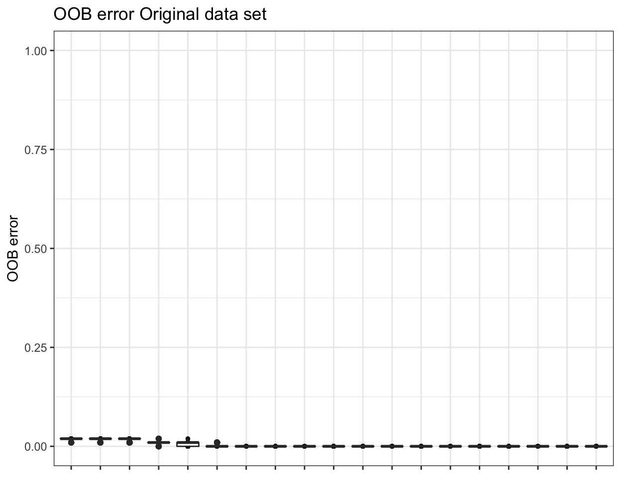
To obtain the confusion matrix from random forests classification use the following:
ssu_prev_confuse <- paste("ssu_best.prev$`Confusion`$", ssu_best, sep = "")
eval(parse(text = (ssu_prev_confuse)))
Save Phyloseq PIME objects
ssu_ps_pime <- ssu_prevalence_best
ssu_ps_pime_tree <- rtree(ntaxa(ssu_ps_pime), rooted = TRUE,
                           tip.label = taxa_names(ssu_ps_pime))
ssu_ps_pime <- merge_phyloseq(ssu_ps_pime,
                               sample_data,
                               ssu_ps_pime_tree)
saveRDS(ssu_ps_pime, "files/trepo/pime/rdata/ssu_ps_merge_otu_pime.rds")
Split & save by predictor variable
ssu_ps_pime_split <- pime.split.by.variable(ssu_ps_pime, "SITE")
saveRDS(ssu_ps_pime_split$ALMR, "files/trepo/pime/rdata/ssu_ps_merge_otu_pime_ALMR.rds")
saveRDS(ssu_ps_pime_split$CRIS, "files/trepo/pime/rdata/ssu_ps_merge_otu_pime_CRIS.rds")
saveRDS(ssu_ps_pime_split$PAST, "files/trepo/pime/rdata/ssu_ps_merge_otu_pime_PAST.rds")
saveRDS(ssu_ps_pime_split$PUCL, "files/trepo/pime/rdata/ssu_ps_merge_otu_pime_PUCL.rds")
$ALMR
phyloseq-class experiment-level object
otu_table() OTU Table: [ 2684 taxa and 26 samples ]
sample_data() Sample Data: [ 26 samples by 6 sample variables ]
tax_table() Taxonomy Table: [ 2684 taxa by 7 taxonomic ranks ]
phy_tree() Phylogenetic Tree: [ 2684 tips and 2683 internal nodes ]
$CRIS
phyloseq-class experiment-level object
otu_table() OTU Table: [ 2699 taxa and 26 samples ]
sample_data() Sample Data: [ 26 samples by 6 sample variables ]
tax_table() Taxonomy Table: [ 2699 taxa by 7 taxonomic ranks ]
phy_tree() Phylogenetic Tree: [ 2699 tips and 2698 internal nodes ]
$PAST
phyloseq-class experiment-level object
otu_table() OTU Table: [ 2702 taxa and 26 samples ]
sample_data() Sample Data: [ 26 samples by 6 sample variables ]
tax_table() Taxonomy Table: [ 2702 taxa by 7 taxonomic ranks ]
phy_tree() Phylogenetic Tree: [ 2702 tips and 2701 internal nodes ]
$PUCL
phyloseq-class experiment-level object
otu_table() OTU Table: [ 2820 taxa and 26 samples ]
sample_data() Sample Data: [ 26 samples by 6 sample variables ]
tax_table() Taxonomy Table: [ 2820 taxa by 7 taxonomic ranks ]
phy_tree() Phylogenetic Tree: [ 2820 tips and 2819 internal nodes ]Create Ampvis2 PIME Object
ssu_otu <- data.frame(t(otu_table(ssu_ps_pime)))
ssu_otu[] <- lapply(ssu_otu, as.numeric)
ssu_otu <- as.matrix(ssu_otu)
ssu_tax <- as.matrix(data.frame(tax_table(ssu_ps_pime)))
ssu_samples <- data.frame(sample_data(ssu_ps_pime))
ssu_ps_amp <- merge_phyloseq(otu_table(ssu_otu, taxa_are_rows = TRUE),
                          tax_table(ssu_tax, ssu_tax),
                          sample_data(ssu_samples))
ssu_amp_otu_pime <- data.frame(otu_table(ssu_ps_amp))
ssu_amp_otu_pime <- ssu_amp_otu_pime %>% tibble::rownames_to_column("OTU")
ssu_amp_tax_pime <- data.frame(tax_table(ssu_ps_amp))
ssu_amp_tax_pime <- ssu_amp_tax_pime %>% tibble::rownames_to_column("OTU")
ssu_amp_tax_pime$ASV_SEQ <- NULL
## THE NEXT COMMAND SHOULD BE REMOVED, THIS IS A TEMP FIX
## BECAUSE OTU_ID'S not INCLUDED FROM OTU WF
ssu_amp_tax_pime$ASV_ID <- ssu_amp_tax_pime$OTU
#########
colnames(ssu_amp_tax_pime)[colnames(ssu_amp_tax_pime) == "ASV_ID"] <- "Species"
ssu_amp_otu_tax_pime <- left_join(ssu_amp_otu_pime, ssu_amp_tax_pime, by = "OTU")
ssu_samp_data_t <- data.frame(ssu_samp_data)
#ssu_samp_data_t[,7:9] <- NULL
ssu_amp_data_pime <- amp_load(ssu_amp_otu_tax_pime, metadata = ssu_samp_data_t)
ssu_diversity_pime <-
amp_alphadiv(
ssu_amp_data_pime,
measure = "observed",
richness = FALSE)
ssu_diversity_pime <-
ssu_diversity_pime %>%
dplyr::rename(
"total_reads" = "Reads",
"total_otus" = "ObservedOTUs")
ssu_diversity_pime$coverage = cut(ssu_diversity_pime$total_reads,
c(0, 5000, 25000, 100000, 200000),
labels = c(
"low (< 5k)", "medium (5-25k)",
"high (25-100k)", "extra_high (> 100k)"))
ssu_diversity_pime <- ssu_diversity_pime[order(ssu_diversity_pime$SamName), ]
ssu_amp_pime <- amp_load(ssu_amp_otu_tax_pime,
metadata = ssu_diversity_pime, tree = ssu_ps_pime_tree)
ssu_samp_pime <- ssu_diversity_pime
ssu_samp_pime <- ssu_samp_pime %>% tibble::remove_rownames()ampvis2 object with 4 elements.
Summary of OTU table:
Samples OTUs Total#Reads Min#Reads Max#Reads
104 5012 1269326 11568 12393
Median#Reads Avg#Reads
12224 12205.06
Assigned taxonomy:
Kingdom Phylum Class Order Family
5012(100%) 4993(99.62%) 5010(99.96%) 5006(99.88%) 5000(99.76%)
Genus Species
5010(99.96%) 5012(100%)
Metadata variables: 9
SamName, SITE, WEEK, REGION, SEASON, REP, total_reads, total_otus, coveragesaveRDS(ssu_amp_pime, "files/trepo/pime/rdata/ssu_merge_otu_amp_pime.rds")Summary
Let’s take a look at a table of sample information. Any header with the _p suffix is the PIME filtered data.
And here is how the data sets changed through the PIME filtering process.
| Description | object name | no. samples | total reads | total otus |
|---|---|---|---|---|
| FULL data set | ssu_ps_work_merge_otu | 104 | 6457054 | 21910 |
| Rarefied data | ssu_pime_ds | 104 | 1339728 | 15619 |
| PIME filtered data | ssu_ps_pime | 104 | 1269326 | 5012 |
| PIME (ALMR) | ssu_ps_pime_ALMR | 26 | 319103 | 2684 |
| PIME (CRIS) | ssu_ps_pime_CRIS | 26 | 316360 | 2699 |
| PIME (PAST) | ssu_ps_pime_PAST | 26 | 315960 | 2702 |
| PIME (PUCL) | ssu_ps_pime_PUCL | 26 | 317903 | 2820 |
All Samples (ASV Data)
We will use PIME (Prevalence Interval for Microbiome Evaluation) to create a filtered data set.
Setup
First, choose a phyloseq object and a sample data frame
ssu_pime_ds <- ssu_ps_work
ssu_which_pime <- "ssu_pime_ds"
ssu_pime_ds@phy_tree <- NULL

### USE THIS TO CREATE NEW SAMPLE VARIABLE FOR SPLITTING
##tmp_samp_data <- sample_data(ssu_pime_ds)
#tmp_samp_data$YR_TREAT <- paste(tmp_samp_data$YEAR, tmp_samp_data$TREAT, sep="_")
#tmp_ps <- merge_phyloseq(ssu_pime_ds, tmp_samp_data)
#ssu_pime_ds <- tmp_ps
#rm(list = ls(pattern = "tmp_"))
phyloseq-class experiment-level object
otu_table() OTU Table: [ 47725 taxa and 304 samples ]
sample_data() Sample Data: [ 304 samples by 6 sample variables ]
tax_table() Taxonomy Table: [ 47725 taxa by 8 taxonomic ranks ]ssu_pime_sample_d <- data.frame(rowSums(otu_table(ssu_pime_ds)))
ssu_pime_sample_d <- ssu_pime_sample_d %>% dplyr::rename(total_reads = 1)
ssu_pime_ds <- rarefy_even_depth(ssu_pime_ds,
sample.size = min(ssu_pime_sample_d$total_reads),
trimOTUs = TRUE, replace = FALSE, rngseed = 119)`set.seed(119)` was used to initialize repeatable random subsampling.
Please record this for your records so others can reproduce.
Try `set.seed(119); .Random.seed` for the full vector
19907 OTUs were removed because they are no longer
present in any sample after random subsampling
phyloseq-class experiment-level object
otu_table()   OTU Table:         [ 27818 taxa and 304 samples ]
sample_data() Sample Data:       [ 304 samples by 6 sample variables ]
tax_table()   Taxonomy Table:    [ 27818 taxa by 8 taxonomic ranks ]
The first step in PIME is to define if the microbial community presents a high relative abundance of taxa with low prevalence, which is considered as noise in PIME analysis. This is calculated by random forests analysis and is the baseline noise detection.
ssu_pime.oob.error <- pime.oob.error(ssu_pime_ds, "SITE")[1] 0.02302632Split by Predictor Variable
data.frame(sample_data(ssu_pime_ds))
ssu_per_variable_obj <- pime.split.by.variable(ssu_pime_ds, "SITE")
ssu_per_variable_obj
Detailed results for splitting by sample variables
$ALMR
phyloseq-class experiment-level object
otu_table()   OTU Table:         [ 12119 taxa and 76 samples ]
sample_data() Sample Data:       [ 76 samples by 6 sample variables ]
tax_table()   Taxonomy Table:    [ 12119 taxa by 8 taxonomic ranks ]

$CRIS
phyloseq-class experiment-level object
otu_table()   OTU Table:         [ 12988 taxa and 76 samples ]
sample_data() Sample Data:       [ 76 samples by 6 sample variables ]
tax_table()   Taxonomy Table:    [ 12988 taxa by 8 taxonomic ranks ]

$PAST
phyloseq-class experiment-level object
otu_table()   OTU Table:         [ 13539 taxa and 76 samples ]
sample_data() Sample Data:       [ 76 samples by 6 sample variables ]
tax_table()   Taxonomy Table:    [ 13539 taxa by 8 taxonomic ranks ]

$PUCL
phyloseq-class experiment-level object
otu_table()   OTU Table:         [ 12939 taxa and 76 samples ]
sample_data() Sample Data:       [ 76 samples by 6 sample variables ]
tax_table()   Taxonomy Table:    [ 12939 taxa by 8 taxonomic ranks ]
Calculate Prevalence Intervals
Using the output of pime.split.by.variable, we calculate the prevalence intervals with the function pime.prevalence. This function estimates the highest prevalence possible (no empty ASV table), calculates prevalence for taxa, starting at 5 maximum prevalence possible (no empty ASV table or dropping samples). After prevalence calculation, each prevalence interval are merged.
ssu_prevalences <- pime.prevalence(ssu_per_variable_obj)
ssu_prevalences
Detailed results for all prevalences intervals
$`5`
phyloseq-class experiment-level object
otu_table()   OTU Table:         [ 11795 taxa and 304 samples ]
sample_data() Sample Data:       [ 304 samples by 6 sample variables ]
tax_table()   Taxonomy Table:    [ 11795 taxa by 8 taxonomic ranks ]

$`10`
phyloseq-class experiment-level object
otu_table()   OTU Table:         [ 7795 taxa and 304 samples ]
sample_data() Sample Data:       [ 304 samples by 6 sample variables ]
tax_table()   Taxonomy Table:    [ 7795 taxa by 8 taxonomic ranks ]

$`15`
phyloseq-class experiment-level object
otu_table()   OTU Table:         [ 5610 taxa and 304 samples ]
sample_data() Sample Data:       [ 304 samples by 6 sample variables ]
tax_table()   Taxonomy Table:    [ 5610 taxa by 8 taxonomic ranks ]

$`20`
phyloseq-class experiment-level object
otu_table()   OTU Table:         [ 4226 taxa and 304 samples ]
sample_data() Sample Data:       [ 304 samples by 6 sample variables ]
tax_table()   Taxonomy Table:    [ 4226 taxa by 8 taxonomic ranks ]

$`25`
phyloseq-class experiment-level object
otu_table()   OTU Table:         [ 3341 taxa and 304 samples ]
sample_data() Sample Data:       [ 304 samples by 6 sample variables ]
tax_table()   Taxonomy Table:    [ 3341 taxa by 8 taxonomic ranks ]

$`30`
phyloseq-class experiment-level object
otu_table()   OTU Table:         [ 2819 taxa and 304 samples ]
sample_data() Sample Data:       [ 304 samples by 6 sample variables ]
tax_table()   Taxonomy Table:    [ 2819 taxa by 8 taxonomic ranks ]

$`35`
phyloseq-class experiment-level object
otu_table()   OTU Table:         [ 2297 taxa and 304 samples ]
sample_data() Sample Data:       [ 304 samples by 6 sample variables ]
tax_table()   Taxonomy Table:    [ 2297 taxa by 8 taxonomic ranks ]

$`40`
phyloseq-class experiment-level object
otu_table()   OTU Table:         [ 1854 taxa and 304 samples ]
sample_data() Sample Data:       [ 304 samples by 6 sample variables ]
tax_table()   Taxonomy Table:    [ 1854 taxa by 8 taxonomic ranks ]

$`45`
phyloseq-class experiment-level object
otu_table()   OTU Table:         [ 1537 taxa and 304 samples ]
sample_data() Sample Data:       [ 304 samples by 6 sample variables ]
tax_table()   Taxonomy Table:    [ 1537 taxa by 8 taxonomic ranks ]

$`50`
phyloseq-class experiment-level object
otu_table()   OTU Table:         [ 1269 taxa and 304 samples ]
sample_data() Sample Data:       [ 304 samples by 6 sample variables ]
tax_table()   Taxonomy Table:    [ 1269 taxa by 8 taxonomic ranks ]

$`55`
phyloseq-class experiment-level object
otu_table()   OTU Table:         [ 1123 taxa and 304 samples ]
sample_data() Sample Data:       [ 304 samples by 6 sample variables ]
tax_table()   Taxonomy Table:    [ 1123 taxa by 8 taxonomic ranks ]

$`60`
phyloseq-class experiment-level object
otu_table()   OTU Table:         [ 962 taxa and 304 samples ]
sample_data() Sample Data:       [ 304 samples by 6 sample variables ]
tax_table()   Taxonomy Table:    [ 962 taxa by 8 taxonomic ranks ]

$`65`
phyloseq-class experiment-level object
otu_table()   OTU Table:         [ 813 taxa and 304 samples ]
sample_data() Sample Data:       [ 304 samples by 6 sample variables ]
tax_table()   Taxonomy Table:    [ 813 taxa by 8 taxonomic ranks ]

$`70`
phyloseq-class experiment-level object
otu_table()   OTU Table:         [ 679 taxa and 304 samples ]
sample_data() Sample Data:       [ 304 samples by 6 sample variables ]
tax_table()   Taxonomy Table:    [ 679 taxa by 8 taxonomic ranks ]

$`75`
phyloseq-class experiment-level object
otu_table()   OTU Table:         [ 551 taxa and 304 samples ]
sample_data() Sample Data:       [ 304 samples by 6 sample variables ]
tax_table()   Taxonomy Table:    [ 551 taxa by 8 taxonomic ranks ]

$`80`
phyloseq-class experiment-level object
otu_table()   OTU Table:         [ 481 taxa and 304 samples ]
sample_data() Sample Data:       [ 304 samples by 6 sample variables ]
tax_table()   Taxonomy Table:    [ 481 taxa by 8 taxonomic ranks ]

$`85`
phyloseq-class experiment-level object
otu_table()   OTU Table:         [ 371 taxa and 304 samples ]
sample_data() Sample Data:       [ 304 samples by 6 sample variables ]
tax_table()   Taxonomy Table:    [ 371 taxa by 8 taxonomic ranks ]

$`90`
phyloseq-class experiment-level object
otu_table()   OTU Table:         [ 264 taxa and 304 samples ]
sample_data() Sample Data:       [ 304 samples by 6 sample variables ]
tax_table()   Taxonomy Table:    [ 264 taxa by 8 taxonomic ranks ]

$`95`
phyloseq-class experiment-level object
otu_table()   OTU Table:         [ 168 taxa and 304 samples ]
sample_data() Sample Data:       [ 304 samples by 6 sample variables ]
tax_table()   Taxonomy Table:    [ 168 taxa by 8 taxonomic ranks ]
Calculate Best Prevalence
Finally, we use the function pime.best.prevalence to calculate the best prevalence. The function uses randomForest to build random forests trees for samples classification and variable importance computation. It performs classifications for each prevalence interval returned by pime.prevalence. Variable importance is calculated, returning the Mean Decrease Accuracy (MDA), Mean Decrease Impurity (MDI), overall and by sample group, and taxonomy for each ASV. PIME keeps the top 30 variables with highest MDA each prevalence level.
set.seed(1911)
ssu_best.prev <- pime.best.prevalence(ssu_prevalences, "SITE")
Interval OOB error rate (%) OTUs Nseqs
1 Prevalence 5% 0.33 11795 768526
2 Prevalence 10% 0 7795 711567
3 Prevalence 15% 0 5610 661834
4 Prevalence 20% 0 4226 617129
5 Prevalence 25% 0 3341 578009
6 Prevalence 30% 0 2819 549694
7 Prevalence 35% 0 2297 515763
8 Prevalence 40% 0 1854 479844
9 Prevalence 45% 0 1537 450527
10 Prevalence 50% 0 1269 423402
11 Prevalence 55% 0 1123 402686
12 Prevalence 60% 0 962 378215
13 Prevalence 65% 0 813 352608
14 Prevalence 70% 0 679 324801
15 Prevalence 75% 0 551 294565
16 Prevalence 80% 0 481 273339
17 Prevalence 85% 0 371 240756
18 Prevalence 90% 0 264 202921
19 Prevalence 95% 0 168 158804ssu_what_is_best <- ssu_best.prev$`OOB error`
ssu_what_is_best[, c(2:4)] <- sapply(ssu_what_is_best[, c(2:4)], as.numeric)
ssu_what_is_best <- ssu_what_is_best %>%
dplyr::rename("OOB_error_rate" = "OOB error rate (%)")
ssu_what_is_best$Interval <- str_replace_all(ssu_what_is_best$Interval, "%", "")
ssu_best <- with(ssu_what_is_best, Interval[which.min(OOB_error_rate)])
ssu_best <- paste("`", ssu_best, "`", sep = "")
ssu_prev_choice <- paste("ssu_best.prev$`Importance`$", ssu_best, sep = "")
ssu_imp_best <- eval(parse(text = (ssu_prev_choice)))Looks like the lowest OOB error rate (%) that retains the most ASVs is 0% from Prevalence 10. We will use this interval.
Best Prevalence Summary
#ssu_imp_best[, 13:14] <- list(NULL)
ssu_imp_best[,(ncol(ssu_imp_best)-1):ncol(ssu_imp_best)] <- list(NULL)
ssu_imp_best <- ssu_imp_best %>% dplyr::rename("ASV_ID" = "SequenceID")
Now we need to create a phyloseq object of ASVs at this cutoff (Prevalence 10).
ssu_best_val <- str_replace_all(ssu_best, "Prevalence ", "")
ssu_best_val <- paste("ssu_prevalences$", ssu_best_val, sep = "")
ssu_prevalence_best <- eval(parse(text = (ssu_best_val)))
saveRDS(ssu_prevalence_best, "rdata/trepo/ssu_asv_prevalence_best.rds")
And look at a summary of the data.
phyloseq-class experiment-level object
otu_table()   OTU Table:         [ 7795 taxa and 304 samples ]
sample_data() Sample Data:       [ 304 samples by 6 sample variables ]
tax_table() Taxonomy Table: [ 7795 taxa by 8 taxonomic ranks ]| Metric | Results |
|---|---|
| Min. number of reads | 2027 |
| Max. number of reads | 2482 |
| Total number of reads | 711567 |
| Average number of reads | 2341 |
| Mean number of reads | 2341 |
| Median number of reads | 2347.5 |
| Total ASVS | 7795 |
| Sparsity | 0.863 |
Estimate Error in Prediction
Using the function pime.error.prediction we can estimate the error in prediction. For each prevalence interval, this function randomizes the samples labels into arbitrary groupings using n random permutations, defined by the bootstrap value. For each, randomized and prevalence filtered, data set the OOB error rate is calculated to estimate whether the original differences in groups of samples occur by chance. Results are in a list containing a table and a box plot summarizing the results.
ssu_randomized <- pime.error.prediction(ssu_pime_ds, "TEMP",
                                          bootstrap = 100, parallel = TRUE,
                                          max.prev = 95)
It is also possible to estimate the variation of OOB error for each prevalence interval filtering. This is done by running the random forests classification for n times, determined by the bootstrap value. The function will return a box plot figure and a table for each classification error.
ssu_replicated.oob.error <- pime.oob.replicate(ssu_prevalences, "SITE",
                                               bootstrap = 100, parallel = FALSE)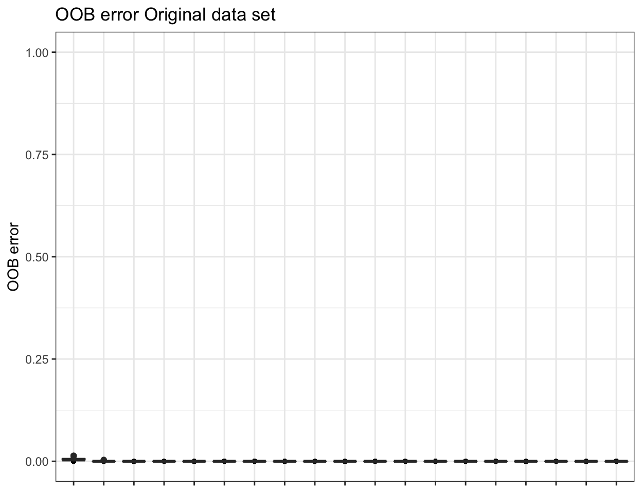
To obtain the confusion matrix from random forests classification use the following:
ssu_prev_confuse <- paste("ssu_best.prev$`Confusion`$", ssu_best, sep = "")
eval(parse(text = (ssu_prev_confuse)))
Save Phyloseq PIME objects
ssu_ps_pime <- ssu_prevalence_best
ssu_ps_pime_tree <- rtree(ntaxa(ssu_ps_pime), rooted = TRUE,
                           tip.label = taxa_names(ssu_ps_pime))
ssu_ps_pime <- merge_phyloseq(ssu_ps_pime,
                               sample_data,
                               ssu_ps_pime_tree)
saveRDS(ssu_ps_pime, "files/trepo/pime/rdata/ssu_ps_asv_pime.rds")
Split & save by predictor variable
ssu_ps_pime_split <- pime.split.by.variable(ssu_ps_pime, "SITE")
saveRDS(ssu_ps_pime_split$ALMR, "files/trepo/pime/rdata/ssu_ps_asv_pime_ALMR.rds")
saveRDS(ssu_ps_pime_split$CRIS, "files/trepo/pime/rdata/ssu_ps_asv_pime_CRIS.rds")
saveRDS(ssu_ps_pime_split$PAST, "files/trepo/pime/rdata/ssu_ps_asv_pime_PAST.rds")
saveRDS(ssu_ps_pime_split$PUCL, "files/trepo/pime/rdata/ssu_ps_asv_pime_PUCL.rds")
$ALMR
phyloseq-class experiment-level object
otu_table() OTU Table: [ 3417 taxa and 76 samples ]
sample_data() Sample Data: [ 76 samples by 6 sample variables ]
tax_table() Taxonomy Table: [ 3417 taxa by 8 taxonomic ranks ]
phy_tree() Phylogenetic Tree: [ 3417 tips and 3416 internal nodes ]
$CRIS
phyloseq-class experiment-level object
otu_table() OTU Table: [ 3336 taxa and 76 samples ]
sample_data() Sample Data: [ 76 samples by 6 sample variables ]
tax_table() Taxonomy Table: [ 3336 taxa by 8 taxonomic ranks ]
phy_tree() Phylogenetic Tree: [ 3336 tips and 3335 internal nodes ]
$PAST
phyloseq-class experiment-level object
otu_table() OTU Table: [ 3471 taxa and 76 samples ]
sample_data() Sample Data: [ 76 samples by 6 sample variables ]
tax_table() Taxonomy Table: [ 3471 taxa by 8 taxonomic ranks ]
phy_tree() Phylogenetic Tree: [ 3471 tips and 3470 internal nodes ]
$PUCL
phyloseq-class experiment-level object
otu_table() OTU Table: [ 3859 taxa and 76 samples ]
sample_data() Sample Data: [ 76 samples by 6 sample variables ]
tax_table() Taxonomy Table: [ 3859 taxa by 8 taxonomic ranks ]
phy_tree() Phylogenetic Tree: [ 3859 tips and 3858 internal nodes ]Create Ampvis2 PIME Object
ssu_otu <- data.frame(t(otu_table(ssu_ps_pime)))
ssu_otu[] <- lapply(ssu_otu, as.numeric)
ssu_otu <- as.matrix(ssu_otu)
ssu_tax <- as.matrix(data.frame(tax_table(ssu_ps_pime)))
ssu_samples <- data.frame(sample_data(ssu_ps_pime))
ssu_ps_amp <- merge_phyloseq(otu_table(ssu_otu, taxa_are_rows = TRUE),
                          tax_table(ssu_tax, ssu_tax),
                          sample_data(ssu_samples))
ssu_amp_asv_pime <- data.frame(otu_table(ssu_ps_amp))
ssu_amp_asv_pime <- ssu_amp_asv_pime %>% tibble::rownames_to_column("OTU")
ssu_amp_tax_pime <- data.frame(tax_table(ssu_ps_amp))
ssu_amp_tax_pime <- ssu_amp_tax_pime %>% tibble::rownames_to_column("OTU")
ssu_amp_tax_pime$ASV_SEQ <- NULL
colnames(ssu_amp_tax_pime)[colnames(ssu_amp_tax_pime) == "ASV_ID"] <- "Species"
ssu_amp_asv_tax_pime <- left_join(ssu_amp_asv_pime, ssu_amp_tax_pime, by = "OTU")
ssu_samp_data_t <- data.frame(ssu_samp_data)
#ssu_samp_data_t[,7:9] <- NULL
ssu_amp_data_pime <- amp_load(ssu_amp_asv_tax_pime, metadata = ssu_samp_data_t)
ssu_diversity_pime <-
amp_alphadiv(
ssu_amp_data_pime,
measure = "observed",
richness = FALSE)
ssu_diversity_pime <-
ssu_diversity_pime %>%
dplyr::rename(
"total_reads" = "Reads",
"total_asvs" = "ObservedOTUs")
ssu_diversity_pime$coverage = cut(ssu_diversity_pime$total_reads,
c(0, 5000, 25000, 100000, 200000),
labels = c(
"low (< 5k)", "medium (5-25k)",
"high (25-100k)", "extra_high (> 100k)"))
ssu_diversity_pime <- ssu_diversity_pime[order(ssu_diversity_pime$SamName), ]
ssu_amp_pime <- amp_load(ssu_amp_asv_tax_pime,
metadata = ssu_diversity_pime, tree = ssu_ps_pime_tree)
ssu_samp_pime <- ssu_diversity_pime
ssu_samp_pime <- ssu_samp_pime %>% tibble::remove_rownames()ampvis2 object with 4 elements.
Summary of OTU table:
Samples OTUs Total#Reads Min#Reads Max#Reads
304 7795 711567 2027 2482
Median#Reads Avg#Reads
2347.5 2340.68
Assigned taxonomy:
Kingdom Phylum Class Order Family
7795(100%) 7786(99.88%) 7794(99.99%) 7791(99.95%) 7775(99.74%)
Genus Species
7795(100%) 7795(100%)
Metadata variables: 9
SamName, SITE, WEEK, REGION, SEASON, REP, total_reads, total_asvs, coveragesaveRDS(ssu_amp_pime, "files/trepo/pime/rdata/ssu_asv_amp_pime.rds")Summary
Let’s take a look at a table of sample information. Any header with the _p suffix is the PIME filtered data.
And here is how the data sets changed through the PIME filtering process.
| Description | object name | no. samples | total reads | total asvs |
|---|---|---|---|---|
| FULL data set | ssu_ps_work | 304 | 6457054 | 47725 |
| Rarefied data | ssu_pime_ds | 304 | 820496 | 27818 |
| PIME filtered data | ssu_ps_pime | 304 | 711567 | 7795 |
| PIME (ALMR) | ssu_ps_pime_ALMR | 76 | 179992 | 3417 |
| PIME (CRIS) | ssu_ps_pime_CRIS | 76 | 176867 | 3336 |
| PIME (PAST) | ssu_ps_pime_PAST | 76 | 175867 | 3471 |
| PIME (PUCL) | ssu_ps_pime_PUCL | 76 | 178841 | 3859 |
All Samples (OTU Data)
We will use PIME (Prevalence Interval for Microbiome Evaluation) to create a filtered data set.
Setup
First, choose a phyloseq object and a sample data frame
ssu_pime_ds <- ssu_ps_work_otu
ssu_which_pime <- "ssu_pime_ds"
ssu_pime_ds@phy_tree <- NULL

### USE THIS TO CREATE NEW SAMPLE VARIABLE FOR SPLITTING
#tmp_samp_data <- sample_data(ssu_pime_ds)
#tmp_samp_data$YR_TREAT <- paste(tmp_samp_data$YEAR, tmp_samp_data$TREAT, sep="_")
#tmp_ps <- merge_phyloseq(ssu_pime_ds, tmp_samp_data)
#ssu_pime_ds <- tmp_ps
#rm(list = ls(pattern = "tmp_"))
phyloseq-class experiment-level object
otu_table() OTU Table: [ 21906 taxa and 304 samples ]
sample_data() Sample Data: [ 304 samples by 6 sample variables ]
tax_table() Taxonomy Table: [ 21906 taxa by 7 taxonomic ranks ]ssu_pime_sample_d <- data.frame(rowSums(otu_table(ssu_pime_ds)))
ssu_pime_sample_d <- ssu_pime_sample_d %>% dplyr::rename(total_reads = 1)
ssu_pime_ds <- rarefy_even_depth(ssu_pime_ds,
sample.size = min(ssu_pime_sample_d$total_reads),
trimOTUs = TRUE, replace = FALSE, rngseed = 119)
ssu_pime_ds`set.seed(119)` was used to initialize repeatable random subsampling.
Please record this for your records so others can reproduce.
Try `set.seed(119); .Random.seed` for the full vector
8456 OTUs were removed because they are no longer
present in any sample after random subsamplingphyloseq-class experiment-level object
otu_table() OTU Table: [ 13450 taxa and 304 samples ]
sample_data() Sample Data: [ 304 samples by 6 sample variables ]
tax_table() Taxonomy Table: [ 13450 taxa by 7 taxonomic ranks ]The first step in PIME is to define if the microbial community presents a high relative abundance of taxa with low prevalence, which is considered as noise in PIME analysis. This is calculated by random forests analysis and is the baseline noise detection.
ssu_pime.oob.error <- pime.oob.error(ssu_pime_ds, "SITE")[1] 0.01644737Split by Predictor Variable
data.frame(sample_data(ssu_pime_ds))
ssu_per_variable_obj <- pime.split.by.variable(ssu_pime_ds, "SITE")
ssu_per_variable_obj
Detailed results for splitting by sample variables
$ALMR
phyloseq-class experiment-level object
otu_table()   OTU Table:         [ 6631 taxa and 76 samples ]
sample_data() Sample Data:       [ 76 samples by 6 sample variables ]
tax_table()   Taxonomy Table:    [ 6631 taxa by 7 taxonomic ranks ]

$CRIS
phyloseq-class experiment-level object
otu_table()   OTU Table:         [ 6995 taxa and 76 samples ]
sample_data() Sample Data:       [ 76 samples by 6 sample variables ]
tax_table()   Taxonomy Table:    [ 6995 taxa by 7 taxonomic ranks ]

$PAST
phyloseq-class experiment-level object
otu_table()   OTU Table:         [ 7174 taxa and 76 samples ]
sample_data() Sample Data:       [ 76 samples by 6 sample variables ]
tax_table()   Taxonomy Table:    [ 7174 taxa by 7 taxonomic ranks ]

$PUCL
phyloseq-class experiment-level object
otu_table()   OTU Table:         [ 6864 taxa and 76 samples ]
sample_data() Sample Data:       [ 76 samples by 6 sample variables ]
tax_table()   Taxonomy Table:    [ 6864 taxa by 7 taxonomic ranks ]
Calculate Prevalence Intervals
Using the output of pime.split.by.variable, we calculate the prevalence intervals with the function pime.prevalence. This function estimates the highest prevalence possible (no empty ASV table), calculates prevalence for taxa, starting at 5 maximum prevalence possible (no empty ASV table or dropping samples). After prevalence calculation, each prevalence interval are merged.
ssu_prevalences <- pime.prevalence(ssu_per_variable_obj)
ssu_prevalences
Detailed results for all prevalences intervals
$`5`
phyloseq-class experiment-level object
otu_table()   OTU Table:         [ 6176 taxa and 304 samples ]
sample_data() Sample Data:       [ 304 samples by 6 sample variables ]
tax_table()   Taxonomy Table:    [ 6176 taxa by 7 taxonomic ranks ]

$`10`
phyloseq-class experiment-level object
otu_table()   OTU Table:         [ 4310 taxa and 304 samples ]
sample_data() Sample Data:       [ 304 samples by 6 sample variables ]
tax_table()   Taxonomy Table:    [ 4310 taxa by 7 taxonomic ranks ]

$`15`
phyloseq-class experiment-level object
otu_table()   OTU Table:         [ 3371 taxa and 304 samples ]
sample_data() Sample Data:       [ 304 samples by 6 sample variables ]
tax_table()   Taxonomy Table:    [ 3371 taxa by 7 taxonomic ranks ]

$`20`
phyloseq-class experiment-level object
otu_table()   OTU Table:         [ 2671 taxa and 304 samples ]
sample_data() Sample Data:       [ 304 samples by 6 sample variables ]
tax_table()   Taxonomy Table:    [ 2671 taxa by 7 taxonomic ranks ]

$`25`
phyloseq-class experiment-level object
otu_table()   OTU Table:         [ 2219 taxa and 304 samples ]
sample_data() Sample Data:       [ 304 samples by 6 sample variables ]
tax_table()   Taxonomy Table:    [ 2219 taxa by 7 taxonomic ranks ]

$`30`
phyloseq-class experiment-level object
otu_table()   OTU Table:         [ 1963 taxa and 304 samples ]
sample_data() Sample Data:       [ 304 samples by 6 sample variables ]
tax_table()   Taxonomy Table:    [ 1963 taxa by 7 taxonomic ranks ]

$`35`
phyloseq-class experiment-level object
otu_table()   OTU Table:         [ 1687 taxa and 304 samples ]
sample_data() Sample Data:       [ 304 samples by 6 sample variables ]
tax_table()   Taxonomy Table:    [ 1687 taxa by 7 taxonomic ranks ]

$`40`
phyloseq-class experiment-level object
otu_table()   OTU Table:         [ 1464 taxa and 304 samples ]
sample_data() Sample Data:       [ 304 samples by 6 sample variables ]
tax_table()   Taxonomy Table:    [ 1464 taxa by 7 taxonomic ranks ]

$`45`
phyloseq-class experiment-level object
otu_table()   OTU Table:         [ 1271 taxa and 304 samples ]
sample_data() Sample Data:       [ 304 samples by 6 sample variables ]
tax_table()   Taxonomy Table:    [ 1271 taxa by 7 taxonomic ranks ]

$`50`
phyloseq-class experiment-level object
otu_table()   OTU Table:         [ 1106 taxa and 304 samples ]
sample_data() Sample Data:       [ 304 samples by 6 sample variables ]
tax_table()   Taxonomy Table:    [ 1106 taxa by 7 taxonomic ranks ]

$`55`
phyloseq-class experiment-level object
otu_table()   OTU Table:         [ 989 taxa and 304 samples ]
sample_data() Sample Data:       [ 304 samples by 6 sample variables ]
tax_table()   Taxonomy Table:    [ 989 taxa by 7 taxonomic ranks ]

$`60`
phyloseq-class experiment-level object
otu_table()   OTU Table:         [ 856 taxa and 304 samples ]
sample_data() Sample Data:       [ 304 samples by 6 sample variables ]
tax_table()   Taxonomy Table:    [ 856 taxa by 7 taxonomic ranks ]

$`65`
phyloseq-class experiment-level object
otu_table()   OTU Table:         [ 747 taxa and 304 samples ]
sample_data() Sample Data:       [ 304 samples by 6 sample variables ]
tax_table()   Taxonomy Table:    [ 747 taxa by 7 taxonomic ranks ]

$`70`
phyloseq-class experiment-level object
otu_table()   OTU Table:         [ 660 taxa and 304 samples ]
sample_data() Sample Data:       [ 304 samples by 6 sample variables ]
tax_table()   Taxonomy Table:    [ 660 taxa by 7 taxonomic ranks ]

$`75`
phyloseq-class experiment-level object
otu_table()   OTU Table:         [ 576 taxa and 304 samples ]
sample_data() Sample Data:       [ 304 samples by 6 sample variables ]
tax_table()   Taxonomy Table:    [ 576 taxa by 7 taxonomic ranks ]

$`80`
phyloseq-class experiment-level object
otu_table()   OTU Table:         [ 514 taxa and 304 samples ]
sample_data() Sample Data:       [ 304 samples by 6 sample variables ]
tax_table()   Taxonomy Table:    [ 514 taxa by 7 taxonomic ranks ]

$`85`
phyloseq-class experiment-level object
otu_table()   OTU Table:         [ 424 taxa and 304 samples ]
sample_data() Sample Data:       [ 304 samples by 6 sample variables ]
tax_table()   Taxonomy Table:    [ 424 taxa by 7 taxonomic ranks ]

$`90`
phyloseq-class experiment-level object
otu_table()   OTU Table:         [ 346 taxa and 304 samples ]
sample_data() Sample Data:       [ 304 samples by 6 sample variables ]
tax_table()   Taxonomy Table:    [ 346 taxa by 7 taxonomic ranks ]

$`95`
phyloseq-class experiment-level object
otu_table()   OTU Table:         [ 243 taxa and 304 samples ]
sample_data() Sample Data:       [ 304 samples by 6 sample variables ]
tax_table()   Taxonomy Table:    [ 243 taxa by 7 taxonomic ranks ]
Calculate Best Prevalence
Finally, we use the function pime.best.prevalence to calculate the best prevalence. The function uses randomForest to build random forests trees for samples classification and variable importance computation. It performs classifications for each prevalence interval returned by pime.prevalence. Variable importance is calculated, returning the Mean Decrease Accuracy (MDA), Mean Decrease Impurity (MDI), overall and by sample group, and taxonomy for each ASV. PIME keeps the top 30 variables with highest MDA each prevalence level.
set.seed(1911)
ssu_best.prev <- pime.best.prevalence(ssu_prevalences, "SITE")
Interval OOB error rate (%) OTUs Nseqs
1 Prevalence 5% 0.99 6176 795077
2 Prevalence 10% 0.33 4310 766467
3 Prevalence 15% 0 3371 740985
4 Prevalence 20% 0 2671 714655
5 Prevalence 25% 0 2219 691362
6 Prevalence 30% 0 1963 674292
7 Prevalence 35% 0 1687 653346
8 Prevalence 40% 0 1464 632093
9 Prevalence 45% 0 1271 611427
10 Prevalence 50% 0 1106 591999
11 Prevalence 55% 0 989 576446
12 Prevalence 60% 0 856 554607
13 Prevalence 65% 0 747 532236
14 Prevalence 70% 0 660 510859
15 Prevalence 75% 0 576 483648
16 Prevalence 80% 0 514 465813
17 Prevalence 85% 0 424 437508
18 Prevalence 90% 0 346 398043
19 Prevalence 95% 0 243 336356ssu_what_is_best <- ssu_best.prev$`OOB error`
ssu_what_is_best[, c(2:4)] <- sapply(ssu_what_is_best[, c(2:4)], as.numeric)
ssu_what_is_best <- ssu_what_is_best %>%
dplyr::rename("OOB_error_rate" = "OOB error rate (%)")
ssu_what_is_best$Interval <- str_replace_all(ssu_what_is_best$Interval, "%", "")
ssu_best <- with(ssu_what_is_best, Interval[which.min(OOB_error_rate)])
ssu_best <- paste("`", ssu_best, "`", sep = "")
ssu_prev_choice <- paste("ssu_best.prev$`Importance`$", ssu_best, sep = "")
ssu_imp_best <- eval(parse(text = (ssu_prev_choice)))Looks like the lowest OOB error rate (%) that retains the most ASVs is 0% from Prevalence 15. We will use this interval.
Best Prevalence Summary
#ssu_imp_best[, 13:14] <- list(NULL)
ssu_imp_best[,(ncol(ssu_imp_best)-1):ncol(ssu_imp_best)] <- list(NULL)
ssu_imp_best <- ssu_imp_best %>% dplyr::rename("ASV_ID" = "SequenceID")
Now we need to create a phyloseq object of ASVs at this cutoff (Prevalence 15).
ssu_best_val <- str_replace_all(ssu_best, "Prevalence ", "")
ssu_best_val <- paste("ssu_prevalences$", ssu_best_val, sep = "")
ssu_prevalence_best <- eval(parse(text = (ssu_best_val)))
saveRDS(ssu_prevalence_best, "rdata/trepo/ssu_otu_prevalence_best.rds")
And look at a summary of the data.
phyloseq-class experiment-level object
otu_table()   OTU Table:         [ 3371 taxa and 304 samples ]
sample_data() Sample Data:       [ 304 samples by 6 sample variables ]
tax_table() Taxonomy Table: [ 3371 taxa by 7 taxonomic ranks ]| Metric | Results |
|---|---|
| Min. number of reads | 2242 |
| Max. number of reads | 2557 |
| Total number of reads | 740985 |
| Average number of reads | 2437 |
| Mean number of reads | 2437 |
| Median number of reads | 2442 |
| Total ASVS | 3371 |
| Sparsity | 0.771 |
Estimate Error in Prediction
Using the function pime.error.prediction we can estimate the error in prediction. For each prevalence interval, this function randomizes the samples labels into arbitrary groupings using n random permutations, defined by the bootstrap value. For each, randomized and prevalence filtered, data set the OOB error rate is calculated to estimate whether the original differences in groups of samples occur by chance. Results are in a list containing a table and a box plot summarizing the results.
ssu_randomized <- pime.error.prediction(ssu_pime_ds, "TEMP",
                                          bootstrap = 100, parallel = TRUE,
                                          max.prev = 95)
It is also possible to estimate the variation of OOB error for each prevalence interval filtering. This is done by running the random forests classification for n times, determined by the bootstrap value. The function will return a box plot figure and a table for each classification error.
ssu_replicated.oob.error <- pime.oob.replicate(ssu_prevalences, "SITE",
                                               bootstrap = 100, parallel = FALSE)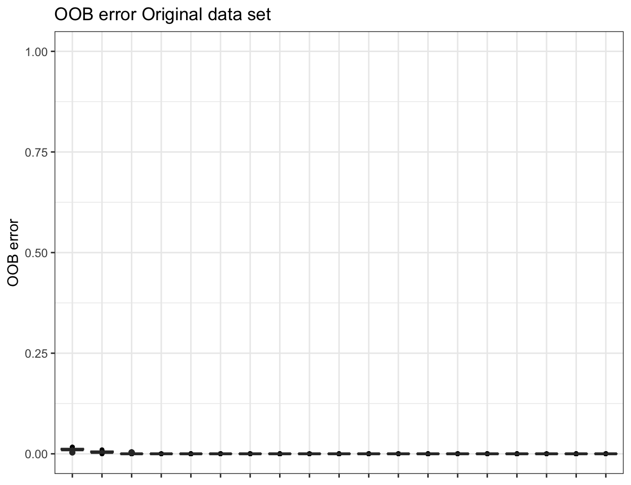
To obtain the confusion matrix from random forests classification use the following:
ssu_prev_confuse <- paste("ssu_best.prev$`Confusion`$", ssu_best, sep = "")
eval(parse(text = (ssu_prev_confuse)))
Save Phyloseq PIME objects
ssu_ps_pime <- ssu_prevalence_best
ssu_ps_pime_tree <- rtree(ntaxa(ssu_ps_pime), rooted = TRUE,
                           tip.label = taxa_names(ssu_ps_pime))
ssu_ps_pime <- merge_phyloseq(ssu_ps_pime,
                               sample_data,
                               ssu_ps_pime_tree)
saveRDS(ssu_ps_pime, "files/trepo/pime/rdata/ssu_ps_otu_pime.rds")
Split & save by predictor variable
ssu_ps_pime_split <- pime.split.by.variable(ssu_ps_pime, "SITE")
saveRDS(ssu_ps_pime_split$ALMR, "files/trepo/pime/rdata/ssu_ps_otu_pime_ALMR.rds")
saveRDS(ssu_ps_pime_split$CRIS, "files/trepo/pime/rdata/ssu_ps_otu_pime_CRIS.rds")
saveRDS(ssu_ps_pime_split$PAST, "files/trepo/pime/rdata/ssu_ps_otu_pime_PAST.rds")
saveRDS(ssu_ps_pime_split$PUCL, "files/trepo/pime/rdata/ssu_ps_otu_pime_PUCL.rds")
$ALMR
phyloseq-class experiment-level object
otu_table() OTU Table: [ 1719 taxa and 76 samples ]
sample_data() Sample Data: [ 76 samples by 6 sample variables ]
tax_table() Taxonomy Table: [ 1719 taxa by 7 taxonomic ranks ]
phy_tree() Phylogenetic Tree: [ 1719 tips and 1718 internal nodes ]
$CRIS
phyloseq-class experiment-level object
otu_table() OTU Table: [ 1713 taxa and 76 samples ]
sample_data() Sample Data: [ 76 samples by 6 sample variables ]
tax_table() Taxonomy Table: [ 1713 taxa by 7 taxonomic ranks ]
phy_tree() Phylogenetic Tree: [ 1713 tips and 1712 internal nodes ]
$PAST
phyloseq-class experiment-level object
otu_table() OTU Table: [ 1771 taxa and 76 samples ]
sample_data() Sample Data: [ 76 samples by 6 sample variables ]
tax_table() Taxonomy Table: [ 1771 taxa by 7 taxonomic ranks ]
phy_tree() Phylogenetic Tree: [ 1771 tips and 1770 internal nodes ]
$PUCL
phyloseq-class experiment-level object
otu_table() OTU Table: [ 1893 taxa and 76 samples ]
sample_data() Sample Data: [ 76 samples by 6 sample variables ]
tax_table() Taxonomy Table: [ 1893 taxa by 7 taxonomic ranks ]
phy_tree() Phylogenetic Tree: [ 1893 tips and 1892 internal nodes ]Create Ampvis2 PIME Object
ssu_otu <- data.frame(t(otu_table(ssu_ps_pime)))
ssu_otu[] <- lapply(ssu_otu, as.numeric)
ssu_otu <- as.matrix(ssu_otu)
ssu_tax <- as.matrix(data.frame(tax_table(ssu_ps_pime)))
ssu_samples <- data.frame(sample_data(ssu_ps_pime))
ssu_ps_amp <- merge_phyloseq(otu_table(ssu_otu, taxa_are_rows = TRUE),
                          tax_table(ssu_tax, ssu_tax),
                          sample_data(ssu_samples))
ssu_amp_otu_pime <- data.frame(otu_table(ssu_ps_amp))
ssu_amp_otu_pime <- ssu_amp_otu_pime %>% tibble::rownames_to_column("OTU")
ssu_amp_tax_pime <- data.frame(tax_table(ssu_ps_amp))
ssu_amp_tax_pime <- ssu_amp_tax_pime %>% tibble::rownames_to_column("OTU")
ssu_amp_tax_pime$ASV_SEQ <- NULL
## THE NEXT COMMAND SHOULD BE REMOVED, THIS IS A TEMP FIX
## BECAUSE OTU_ID'S not INCLUDED FROM OTU WF
ssu_amp_tax_pime$ASV_ID <- ssu_amp_tax_pime$OTU
#########
colnames(ssu_amp_tax_pime)[colnames(ssu_amp_tax_pime) == "ASV_ID"] <- "Species"
ssu_amp_otu_tax_pime <- left_join(ssu_amp_otu_pime, ssu_amp_tax_pime, by = "OTU")
ssu_samp_data_t <- data.frame(ssu_samp_data)
#ssu_samp_data_t[,7:9] <- NULL
ssu_amp_data_pime <- amp_load(ssu_amp_otu_tax_pime, metadata = ssu_samp_data_t)
ssu_diversity_pime <-
amp_alphadiv(
ssu_amp_data_pime,
measure = "observed",
richness = FALSE)
ssu_diversity_pime <-
ssu_diversity_pime %>%
dplyr::rename(
"total_reads" = "Reads",
"total_otus" = "ObservedOTUs")
ssu_diversity_pime$coverage = cut(ssu_diversity_pime$total_reads,
c(0, 5000, 25000, 100000, 200000),
labels = c(
"low (< 5k)", "medium (5-25k)",
"high (25-100k)", "extra_high (> 100k)"))
ssu_diversity_pime <- ssu_diversity_pime[order(ssu_diversity_pime$SamName), ]
ssu_amp_pime <- amp_load(ssu_amp_otu_tax_pime,
metadata = ssu_diversity_pime, tree = ssu_ps_pime_tree)
ssu_samp_pime <- ssu_diversity_pime
ssu_samp_pime <- ssu_samp_pime %>% tibble::remove_rownames()ampvis2 object with 4 elements.
Summary of OTU table:
Samples OTUs Total#Reads Min#Reads Max#Reads
304 3371 740985 2242 2557
Median#Reads Avg#Reads
2442 2437.45
Assigned taxonomy:
Kingdom Phylum Class Order Family
3371(100%) 3364(99.79%) 3370(99.97%) 3367(99.88%) 3365(99.82%)
Genus Species
3371(100%) 3371(100%)
Metadata variables: 9
SamName, SITE, WEEK, REGION, SEASON, REP, total_reads, total_otus, coveragesaveRDS(ssu_amp_pime, "files/trepo/pime/rdata/ssu_otu_amp_pime.rds")Summary
Let’s take a look at a table of sample information. Any header with the _p suffix is the PIME filtered data.
And here is how the data sets changed through the PIME filtering process.
| Description | object name | no. samples | total reads | total otus |
|---|---|---|---|---|
| FULL data set | ssu_ps_work_otu | 304 | 6457054 | 21906 |
| Rarefied data | ssu_pime_ds | 304 | 820496 | 13450 |
| PIME filtered data | ssu_ps_pime | 304 | 740985 | 3371 |
| PIME (ALMR) | ssu_ps_pime_ALMR | 76 | 186549 | 1719 |
| PIME (CRIS) | ssu_ps_pime_CRIS | 76 | 184235 | 1713 |
| PIME (PAST) | ssu_ps_pime_PAST | 76 | 184770 | 1771 |
| PIME (PUCL) | ssu_ps_pime_PUCL | 76 | 185431 | 1893 |
Source Code
The source code for this page can be accessed on GitHub by clicking this link. Please note, that in order to process the data and build the website, we needed to run the workflow and get the results. Then hard code the results and turn off the individual commands. So the raw file for this page is a bit messy—you have been warned.