Hit the Hide Code button to hide the R code.
Synopsis
This workflow contains beta diversity assessments. In order to run the workflow, you either need to first run the DADA2 Workflow and the Data Preparation workflow or begin with the output files from the Data Preparation workflow. See the Data Availability page for complete details.
In this workflow…
Full Data Set
Significance Tests
In order to test for significance between sample groups, we must perform the following steps:
- Create distance matrices based on the metrics above (
wunifrac,unifrac,jsd). For this we use the functionphyloseq::distance. - Next, calculate beta dispersion using the
betadisperfunction from theveganpackage. - Then, use the function
permutestto run a Permutation test for homogeneity of multivariate dispersions. - If the beta dispersion tests are not significant we will run a PERMANOVA (since PERMANOVA assumes equal dispersion), otherwise we will use Analysis of Similarity (ANOSIM).
Steps 1, 2, and 3 are analyzed in a for loop that tests all three distance metrics.
Before we begin, we must first transform sample counts to relative abundance for both data sets.
samp_ps <- c("ssu_ps_work", "ssu_ps_pime")
for (i in samp_ps) {
     tmp_name <- purrr::map_chr(i, ~ paste0(., "_prop"))
     tmp_get <- get(i)
     tmp_ps <- transform_sample_counts(tmp_get, function(otu) 1E6 * otu/sum(otu))
     tmp_ps@phy_tree <- NULL
     tmp_ps <- prune_samples(sample_sums(tmp_ps) > 0, tmp_ps)
     tmp_tree <- rtree(ntaxa(tmp_ps), rooted = TRUE, tip.label = taxa_names(tmp_ps))
     tmp_ps <- merge_phyloseq(tmp_ps, sample_data, tmp_tree)
     print(tmp_name)
     assign(tmp_name, tmp_ps)
     rm(list = ls(pattern = "tmp_"))
}
Beta Dispersion
dist <- c("jsd", "unifrac", "wunifrac")
for (i in samp_ps) {
        for (d in dist){
             tmp_get <- get(purrr::map_chr(i, ~ paste0(i, "_prop")))
             tmp_samp <- data.frame(sample_data(tmp_get))
             tmp_df <- phyloseq::distance(tmp_get, method = d)
             tmp_df_name <- purrr::map_chr(d, ~ paste0(i, "_beta_dist_", .))
             assign(tmp_df_name, tmp_df)
             tmp_df2 <- betadisper(tmp_df, tmp_samp$SITE, bias.adjust = TRUE)
             tmp_df_name2 <- purrr::map_chr(d, ~ paste0(i, "_beta_dispersion_", .))
             assign(tmp_df_name2, tmp_df2)
             tmp_df3 <- permutest(tmp_df2, pairwise = TRUE,
                                  permutations = 1000, binary = FALSE)
             tmp_df_name3 <- purrr::map_chr(d, ~ paste0(i, "_permutest_", .))
             assign(tmp_df_name3, tmp_df3)
             rm(list = ls(pattern = "tmp_"))
       }
}
objects()
Detailed results of Beta Dispersion & Permutation tests
Permutation tests (ASV)
            ***** ssu_ps_work *****

####################################################
BETA DISPERSION significance test jsd distance
####################################################

Permutation test for homogeneity of multivariate dispersions
Permutation: free
Number of permutations: 1000

Response: Distances
           Df  Sum Sq  Mean Sq     F N.Perm   Pr(>F)
Groups      3 0.06601 0.022003 10.02   1000 0.000999 ***
Residuals 300 0.65879 0.002196
---
Signif. codes:  0 '***' 0.001 '**' 0.01 '*' 0.05 '.' 0.1 ' ' 1

Pairwise comparisons:
(Observed p-value below diagonal, permuted p-value above
diagonal)
             ALMR         CRIS         PAST   PUCL
ALMR              0.0009990010 0.0009990010 0.0010
CRIS 0.0000040144              0.4655344655 0.5145
PAST 0.0003331539 0.4580143926              0.2068
PUCL 0.0000031398 0.5088286342 0.2029848564

####################################################
BETA DISPERSION significance test unifrac distance
####################################################

Permutation test for homogeneity of multivariate dispersions
Permutation: free
Number of permutations: 1000

Response: Distances
           Df  Sum Sq   Mean Sq      F N.Perm  Pr(>F)
Groups      3 0.03211 0.0107023 4.1671   1000 0.01099 *
Residuals 300 0.77049 0.0025683
---
Signif. codes:  0 '***' 0.001 '**' 0.01 '*' 0.05 '.' 0.1 ' ' 1

Pairwise comparisons:
(Observed p-value below diagonal, permuted p-value above
diagonal)
           ALMR       CRIS       PAST   PUCL
ALMR            0.00099900 0.02197802 0.0440
CRIS 0.00069814            0.25574426 0.2158
PAST 0.01829183 0.28214168            0.8601
PUCL 0.04063699 0.23952345 0.85615514

####################################################
BETA DISPERSION significance test wunifrac distance
####################################################

Permutation test for homogeneity of multivariate dispersions
Permutation: free
Number of permutations: 1000

Response: Distances
           Df   Sum Sq   Mean Sq      F N.Perm   Pr(>F)
Groups      3 0.011834 0.0039447 4.3124   1000 0.005994 **
Residuals 300 0.274416 0.0009147
---
Signif. codes:  0 '***' 0.001 '**' 0.01 '*' 0.05 '.' 0.1 ' ' 1

Pairwise comparisons:
(Observed p-value below diagonal, permuted p-value above
diagonal)
          ALMR      CRIS      PAST   PUCL
ALMR           0.0019980 0.0059940 0.0020
CRIS 0.0016073           0.8711289 0.8891
PAST 0.0049908 0.8836520           0.7862
PUCL 0.0029881 0.8854266 0.7879608

            ***** ssu_ps_pime *****

####################################################
BETA DISPERSION significance test jsd distance
####################################################

Permutation test for homogeneity of multivariate dispersions
Permutation: free
Number of permutations: 1000

Response: Distances
           Df   Sum Sq   Mean Sq      F N.Perm   Pr(>F)
Groups      3 0.036789 0.0122629 29.194   1000 0.000999 ***
Residuals 300 0.126016 0.0004201
---
Signif. codes:  0 '***' 0.001 '**' 0.01 '*' 0.05 '.' 0.1 ' ' 1

Pairwise comparisons:
(Observed p-value below diagonal, permuted p-value above
diagonal)
                         ALMR                     CRIS
ALMR                          0.0589410589410589436099
CRIS 0.0492723537862556834610
PAST 0.0001881309224778698105 0.0161078666106647255818
PUCL 0.0000000000000000021297 0.0000000000000057418658
                         PAST  PUCL
ALMR 0.0009990009990009990001 0.001
CRIS 0.0159840159840159840021 0.001
PAST                          0.001
PUCL 0.0001432830151268239100

####################################################
BETA DISPERSION significance test unifrac distance
####################################################

Permutation test for homogeneity of multivariate dispersions
Permutation: free
Number of permutations: 1000

Response: Distances
           Df   Sum Sq    Mean Sq      F N.Perm   Pr(>F)
Groups      3 0.008628 0.00287585 6.9188   1000 0.000999 ***
Residuals 300 0.124697 0.00041566
---
Signif. codes:  0 '***' 0.001 '**' 0.01 '*' 0.05 '.' 0.1 ' ' 1

Pairwise comparisons:
(Observed p-value below diagonal, permuted p-value above
diagonal)
             ALMR         CRIS         PAST   PUCL
ALMR              0.0329670330 0.0049950050 0.0010
CRIS 0.0295554789              0.4445554446 0.0130
PAST 0.0057829642 0.4685734650              0.1229
PUCL 0.0000028596 0.0146358858 0.1153458947

####################################################
BETA DISPERSION significance test wunifrac distance
####################################################

Permutation test for homogeneity of multivariate dispersions
Permutation: free
Number of permutations: 1000

Response: Distances
           Df   Sum Sq    Mean Sq      F N.Perm   Pr(>F)
Groups      3 0.002575 0.00085833 4.0231   1000 0.008991 **
Residuals 300 0.064005 0.00021335
---
Signif. codes:  0 '***' 0.001 '**' 0.01 '*' 0.05 '.' 0.1 ' ' 1

Pairwise comparisons:
(Observed p-value below diagonal, permuted p-value above
diagonal)
          ALMR      CRIS      PAST   PUCL
ALMR           0.5264735 0.0089910 0.0170
CRIS 0.5336665           0.0209790 0.0699
PAST 0.0065328 0.0257913           0.4126
PUCL 0.0138408 0.0661387 0.4159449
Remember, if the beta dispersion p-value is greater than 0.05 we use PERMANOVA, otherwise we use ANOSIM.
file.remove("files/trepo/beta/tables/tmp.txt")
for (i in samp_ps) {
        for (d in dist){
          tmp_get <- get(purrr::map_chr(i, ~ paste0(., "_permutest_", d)))
          tmp_res <- eval(isTRUE(tmp_get$tab$`Pr(>F)`[1] < 0.05))
          tmp_print <- c("Permutation test p-value of  ", i, d,
          " < 0.05?", tmp_res)
          cat(tmp_print,"\n", append = TRUE, file = "files/trepo/beta/tables/tmp.txt")
          rm(list = ls(pattern = "tmp_"))
        }
}
ssu_perm_pvalues <- read_delim("files/trepo/beta/tables/tmp.txt",
                               delim = "\n", col_names = "permutation results")
Significance Tests (ALL ASVs)
# A tibble: 3 x 1
  `permutation results`
  <chr>
1 "Permutation test p-value of   ssu_ps_work jsd  < 0.05? TRUE "
2 "Permutation test p-value of   ssu_ps_work unifrac  < 0.05? TRUE "
3 "Permutation test p-value of   ssu_ps_work wunifrac  < 0.05? TRUE "
ssu_ps_work_groups <- get_variable(anosim_data, "SITE")
ssu_ps_work_anosim_jsd <-
anosim(phyloseq::distance(ssu_ps_work_prop, "jsd"),
grouping = ssu_ps_work_groups)ssu_ps_work_groups <- get_variable(anosim_data, "SITE")
ssu_ps_work_anosim_unifrac <-
anosim(phyloseq::distance(ssu_ps_work_prop, "unifrac"),
grouping = ssu_ps_work_groups)ssu_ps_work_groups <- get_variable(anosim_data, "SITE")
ssu_ps_work_anosim_wunifrac <-
anosim(phyloseq::distance(ssu_ps_work_prop, "wunifrac"),
grouping = ssu_ps_work_groups)Detailed results of Significance tests for the ALL ASV data set
***ANOSIM for Jensen-Shannon Divergence, `jsd`***
Call:
anosim(x = phyloseq::distance(ssu_ps_work_prop, "jsd"), grouping = ssu_ps_work_groups)
Dissimilarity:

ANOSIM statistic R: 0.8165
      Significance: 0.001

Permutation: free
Number of permutations: 999

Upper quantiles of permutations (null model):
    90%     95%   97.5%     99%
0.00693 0.01054 0.01422 0.01879

Dissimilarity ranks between and within classes:
        0%     25%     50%      75%  100%     N
Between 34 19411.5 28728.5 37392.25 46056 34656
ALMR     3  1266.5  3664.5  7671.75 22876  2850
CRIS    33  6132.5  9734.5 13611.75 26480  2850
PAST     1  3913.5  8208.0 13723.50 26994  2850
PUCL     6  6351.5 11386.0 15690.75 25006  2850
***ANOSIM for Unweighted UniFrac distance, `unifrac`***
Call:
anosim(x = phyloseq::distance(ssu_ps_work_prop, "unifrac"), grouping = ssu_ps_work_groups)
Dissimilarity:

ANOSIM statistic R: 0.7113
      Significance: 0.001

Permutation: free
Number of permutations: 999

Upper quantiles of permutations (null model):
    90%     95%   97.5%     99%
0.00693 0.00981 0.01266 0.01597

Dissimilarity ranks between and within classes:
        0%      25%     50%      75%  100%     N
Between 27 18308.75 28274.5 37235.25 46056 34656
ALMR    14  1697.25  6373.5 12299.75 45570  2850
CRIS    60  7200.00 11348.0 16306.00 45905  2850
PAST     1  4608.75  9468.5 14801.75 46023  2850
PUCL     2  3960.75  9532.5 16264.75 45641  2850
***ANOSIM for Weighted-UniFrac distance, `wunifrac`***
Call:
anosim(x = phyloseq::distance(ssu_ps_work_prop, "wunifrac"),      grouping = ssu_ps_work_groups)
Dissimilarity:

ANOSIM statistic R: 0.8238
      Significance: 0.001

Permutation: free
Number of permutations: 999

Upper quantiles of permutations (null model):
    90%     95%   97.5%     99%
0.00869 0.01175 0.01520 0.02001

Dissimilarity ranks between and within classes:
         0%      25%     50%      75%  100%     N
Between 195 19191.50 28722.5 37392.25 46056 34656
ALMR      4  1640.25  4403.0  8986.25 24992  2850
CRIS     21  4949.00  8793.0 13249.50 30120  2850
PAST      1  3730.25  8439.0 14273.50 30286  2850
PUCL      3  4515.75  9375.5 14566.50 29327  2850
Significance Tests (PIME ASVs)
# A tibble: 3 x 1
  `permutation results`
  <chr>
1 "Permutation test p-value of   ssu_ps_pime jsd  < 0.05? TRUE "
2 "Permutation test p-value of   ssu_ps_pime unifrac  < 0.05? TRUE "
3 "Permutation test p-value of   ssu_ps_pime wunifrac  < 0.05? TRUE "
ssu_ps_pime_groups <- get_variable(anosim_data, "SITE")
ssu_ps_pime_anosim_jsd <-
anosim(phyloseq::distance(ssu_ps_pime_prop, "jsd"),
grouping = ssu_ps_pime_groups)ssu_ps_pime_groups <- get_variable(anosim_data, "SITE")
ssu_ps_pime_anosim_unifrac <-
anosim(phyloseq::distance(ssu_ps_pime_prop, "unifrac"),
grouping = ssu_ps_pime_groups)ssu_ps_pime_groups <- get_variable(anosim_data, "SITE")
ssu_ps_pime_anosim_wunifrac <-
anosim(phyloseq::distance(ssu_ps_pime_prop, "wunifrac"),
grouping = ssu_ps_pime_groups)Detailed results of Significance tests for PIME data set
***ANOSIM for Jensen-Shannon Divergence, `jsd`***
Call:
anosim(x = phyloseq::distance(ssu_ps_pime_prop, "jsd"), grouping = ssu_ps_pime_groups)
Dissimilarity:

ANOSIM statistic R: 0.8905
      Significance: 0.001

Permutation: free
Number of permutations: 999

Upper quantiles of permutations (null model):
    90%     95%   97.5%     99%
0.00788 0.01097 0.01526 0.01977

Dissimilarity ranks between and within classes:
          0%      25%     50%      75%  100%     N
Between  679 19874.75 28728.5 37392.25 46056 34656
ALMR       1  1009.50  2746.0  6068.00 22760  2850
CRIS     163  3136.75  4835.5  7411.75 21666  2850
PAST       7  2738.25  5902.5 13069.00 26533  2850
PUCL    2905 10087.50 12235.5 14355.75 21756  2850
***ANOSIM for Unweighted UniFrac distance, `unifrac`***
Call:
anosim(x = phyloseq::distance(ssu_ps_pime_prop, "unifrac"), grouping = ssu_ps_pime_groups)
Dissimilarity:

ANOSIM statistic R: 0.8999
      Significance: 0.001

Permutation: free
Number of permutations: 999

Upper quantiles of permutations (null model):
    90%     95%   97.5%     99%
0.00819 0.01134 0.01627 0.02187

Dissimilarity ranks between and within classes:
          0%      25%     50%      75%  100%     N
Between 1025 19680.75 28728.5 37392.25 46056 34656
ALMR       1  1474.50  3703.5  7350.25 21728  2850
CRIS      43  3062.50  5850.5 10042.00 22127  2850
PAST       3  2521.50  6287.5 12541.50 27034  2850
PUCL     417  5948.25  9031.5 12674.75 23433  2850
***ANOSIM for Weighted-UniFrac distance, `wunifrac`***
Call:
anosim(x = phyloseq::distance(ssu_ps_pime_prop, "wunifrac"),      grouping = ssu_ps_pime_groups)
Dissimilarity:

ANOSIM statistic R: 0.8928
      Significance: 0.001

Permutation: free
Number of permutations: 999

Upper quantiles of permutations (null model):
    90%     95%   97.5%     99%
0.00757 0.01112 0.01482 0.02063

Dissimilarity ranks between and within classes:
         0%      25%     50%      75%  100%     N
Between 204 19617.75 28724.5 37392.25 46056 34656
ALMR      1  1575.50  4401.5  9121.50 25690  2850
CRIS     11  2710.75  5299.5  9662.75 25182  2850
PAST      3  3311.25  7608.0 14107.00 33336  2850
PUCL    244  5101.75  8088.5 11271.25 23137  2850
Summary
Here is a quick summary of significance tests for the FULL and PIME ASV data sets against the three distance matrices.
| distance metric | p-value (ALL) | p-value (PIME) |
|---|---|---|
| Jensen-Shannon Divergence | 0.001 | 0.001 |
| unweighted UniFrac | 0.001 | 0.001 |
| weighted UniFrac | 0.001 | 0.001 |
Summary of significant tests for the ALL ASVs and PIME ASVs data sets.
Beta Diversity Plots
This is code in progress. No peaking
source("hack_code/phyloseq_to_ampvis2.R")

tmp_otu <- data.frame(t(otu_table(ssu_ps_work)))
tmp_otu[] <- lapply(tmp_otu, as.numeric)
tmp_otu <- as.matrix(tmp_otu)
tmp_tax <- as.matrix(data.frame(tax_table(ssu_ps_work)))
tmp_samp <- data.frame(sample_data(ssu_ps_work))
ssu_ps_amp <- merge_phyloseq(otu_table(tmp_otu, taxa_are_rows = TRUE),
                          tax_table(tmp_tax, tmp_tax),
                          sample_data(tmp_samp))

tmp_amp_asv_pime  <- data.frame(otu_table(ssu_ps_amp))
tmp_amp_asv_pime <- tmp_amp_asv_pime %>% tibble::rownames_to_column("OTU")
tmp_amp_tax_pime  <- data.frame(tax_table(ssu_ps_amp))
tmp_amp_tax_pime <- tmp_amp_tax_pime %>% tibble::rownames_to_column("OTU")
tmp_amp_tax_pime$ASV_SEQ <- NULL
colnames(tmp_amp_tax_pime)[colnames(tmp_amp_tax_pime) == "ASV_ID"] <- "Species"
tmp_amp_asv_tax_pime <- left_join(tmp_amp_asv_pime, tmp_amp_tax_pime, by = "OTU")
tmp_samp_data_t <- data.frame(sample_data(ssu_ps_amp))
ssu_amp_work <- amp_load(tmp_amp_asv_tax_pime, metadata = tmp_samp_data_t, tree = phy_tree(ssu_ps_work))
tmp_select <- ssu_amp_work
tmp_select$metadata$SITE <- factor(tmp_select$metadata$SITE,
levels = c("ALMR", "PAST", "CRIS", "PUCL"))
ssu_amp_work <- tmp_selectswel_col <- c("#CC79A7", "#E69F00", "#0072B2", "#56B4E9")
amp_ordinate(
ssu_amp_work,
filter_species = 0.1,
type = "PCoA",
distmeasure = "wunifrac",
transform = "none",
constrain = NULL,
x_axis = 1,
y_axis = 2,
print_caption = FALSE,
sample_color_by = "SITE",
sample_color_order = NULL,
sample_shape_by = NULL,
sample_colorframe = FALSE,
sample_colorframe_label = NULL,
sample_colorframe_label_size = 3,
sample_label_by = NULL,
sample_label_size = 4,
sample_label_segment_color = "black",
sample_point_size = 2,
sample_trajectory = NULL,
sample_trajectory_group = NULL,
sample_plotly = NULL,
species_plot = FALSE,
species_nlabels = 0,
species_label_taxonomy = "Genus",
species_label_size = 3,
species_label_color = "grey10",
species_rescale = FALSE,
species_point_size = 2,
species_shape = 20,
species_plotly = FALSE,
envfit_factor = NULL,
envfit_numeric = NULL,
envfit_signif_level = 0.005,
envfit_textsize = 3,
envfit_textcolor = "darkred",
envfit_numeric_arrows_scale = 1,
envfit_arrowcolor = "darkred",
envfit_show = TRUE,
repel_labels = TRUE,
opacity = 0.8,
tax_empty = "best",
detailed_output = FALSE
) + scale_colour_manual(values = swel_col) Here we visualize the different distance matrices using several ordination methods on the ALL and PIME filtered data sets to access dissimilarity among sample.
Plots ALL ASVs
First, we inspect different ordination methods to see how the samples cluster using weighted-UniFrac, unweighted-UniFrac, and Jensen-Shannon Divergence distance measurements. We could also test different diversity metrics, different transformations, etc.
samp_ps <- "ssu_ps_work"
dist <- c("wunifrac", "unifrac", "jsd")
for (d in dist){
     tmp_name <- purrr::map_chr(d, ~ paste0(samp_ps, "_dist_", .))
     tmp_name_plot <- purrr::map_chr(d, ~ paste0(samp_ps, "_dist_", ., "_plot"))
     tmp_get <- get(purrr::map_chr(samp_ps, ~ paste0(., "_prop")))
     ord_meths <- c("NMDS", "PCoA", "CCA", "DCA") #    MDS = PCoA, "CCA", "DCA", "DPCoA", "RDA"
     tmp_plist_name <- purrr::map_chr(d, ~ paste0(samp_ps, "_", ., "_plist"))
     tmp_plist <- llply(as.list(ord_meths), function(i, physeq, d) {
        ordi = ordinate(physeq, method = i, distance = d)
        plot_ordination(physeq, ordi, "samples", color = "SITE")
   }, tmp_get, d)

  names(tmp_plist) <- ord_meths

  tmp_df <- ldply(tmp_plist, function(x){
      df = x$data[, 1:2]
      colnames(df) = c("Axis_1", "Axis_2")
      return(cbind(df, x$data))})
  names(tmp_df)[1] = "method"

  ## NEXT  LINE REORDER FACTORS
  tmp_df$SITE <- factor(tmp_df$SITE, levels = c("ALMR", "PAST", "CRIS", "PUCL"))
  tmp_plot <- ggplot(tmp_df, aes(Axis_1, Axis_2,
                                 color = SITE, shape = SEASON, fill = SITE))
  tmp_plot <- tmp_plot + geom_point(size = 2)
  tmp_plot <- tmp_plot + facet_wrap(~method, scales = "free")
  tmp_plot <- tmp_plot + scale_colour_manual(values = swel_col)
  assign(tmp_plist_name, tmp_plist)
  assign(tmp_name, tmp_df)
  assign(tmp_name_plot, tmp_plot)
  rm(list = ls(pattern = "tmp_"))
}

objects(pattern = "_dist_")
objects()
samp_ps <- "ssu_ps_work"
plist_name <- objects(pattern="_plist")
plot_num <- c(1,2)
for (i in plist_name) {
for (j in plot_num) {
tmp_get_i <- get(i)
## NEXT LINE REORDER FACTORS
tmp_get_i[[j]]$data$SITE <- factor(tmp_get_i[[j]]$data$SITE,
levels = c("ALMR", "PAST", "CRIS", "PUCL"))
tmp_ord <- names(tmp_get_i)[j]
tmp_name <- stringr::str_replace(i, "plist", tmp_ord)
tmp_plot <- tmp_get_i[[j]] + scale_colour_manual(values = swel_col)
tmp_plot <- tmp_plot + geom_point(size = 4, aes(shape = SEASON)) +
theme(legend.position = "bottom")
tmp_plot$labels$shape <- "SEASON"
assign(tmp_name, tmp_plot)
rm(list = ls(pattern = "tmp_"))
}
}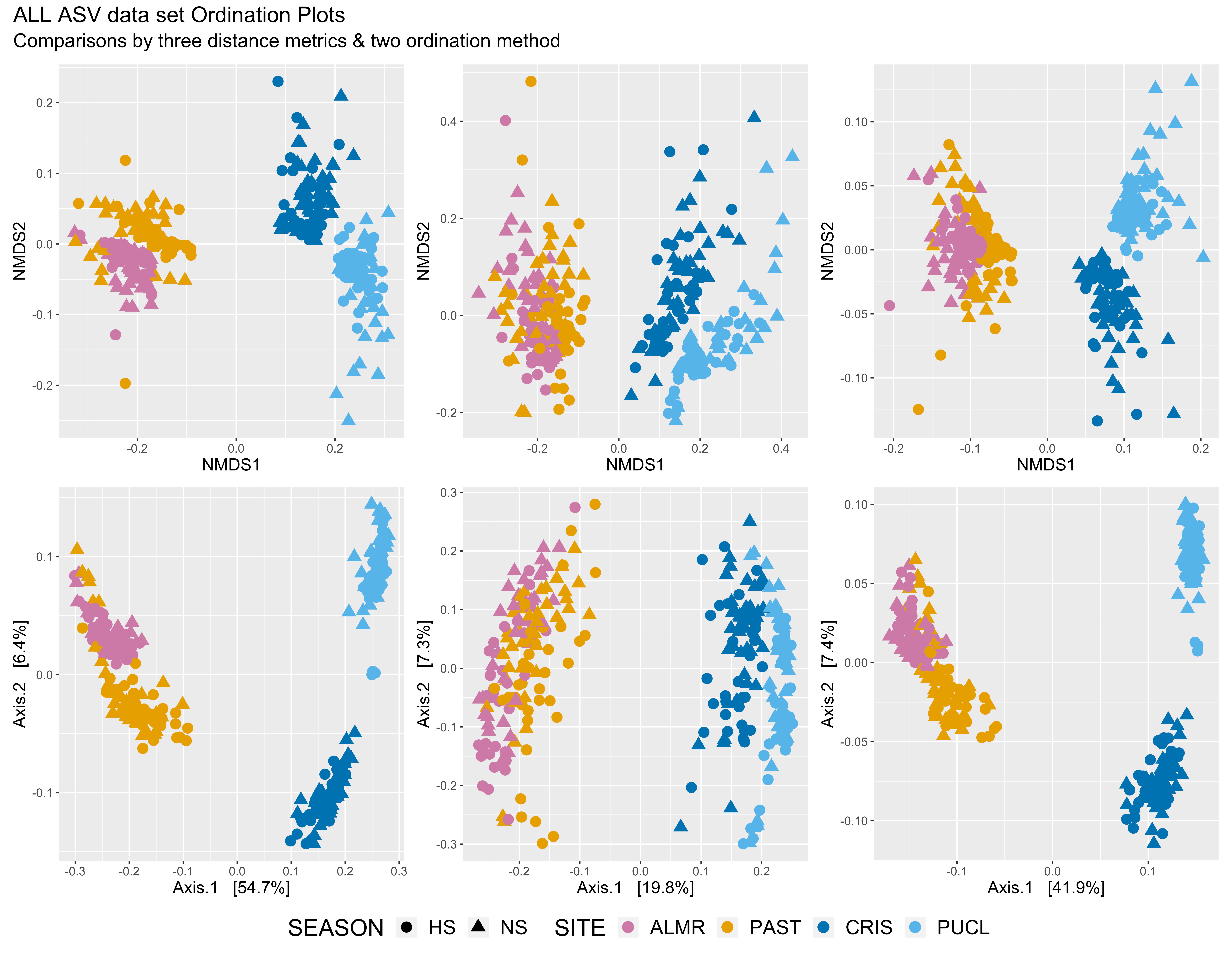
Figure 1: Left = Jensen-Shannon Divergence, middle = UniFrac (unwieghted), right = UniFrac (wieghted); Top = NMDS, bottom = PCoA.
Plots ALL PIME ASV
Same as above, we inspect different ordination methods to see how the samples cluster using weighted-UniFrac, unweighted-UniFrac, and Jensen-Shannon Divergence distance measurements.
samp_ps <- "ssu_ps_pime"
dist <- c("wunifrac", "unifrac", "jsd")
for (d in dist){
     tmp_name <- purrr::map_chr(d, ~ paste0(samp_ps, "_dist_", .))
     tmp_name_plot <- purrr::map_chr(d, ~ paste0(samp_ps, "_dist_", ., "_plot"))
     tmp_get <- get(purrr::map_chr(samp_ps, ~ paste0(., "_prop")))
     ord_meths <- c("NMDS", "PCoA", "CCA", "DCA") #    MDS = PCoA, "CCA", "DCA", "DPCoA", "RDA"
     tmp_plist_name <- purrr::map_chr(d, ~ paste0(samp_ps, "_", ., "_plist"))
     tmp_plist <- llply(as.list(ord_meths), function(i, physeq, d) {
        ordi = ordinate(physeq, method = i, distance = d)
        plot_ordination(physeq, ordi, "samples", color = "SITE")
   }, tmp_get, d)

  names(tmp_plist) <- ord_meths

  tmp_df <- ldply(tmp_plist, function(x){
      df = x$data[, 1:2]
      colnames(df) = c("Axis_1", "Axis_2")
      return(cbind(df, x$data))})
  names(tmp_df)[1] = "method"

  ## NEXT  LINE REORDER FACTORS
  tmp_df$SITE <- factor(tmp_df$SITE, levels = c("ALMR", "PAST", "CRIS", "PUCL"))
  tmp_plot <- ggplot(tmp_df, aes(Axis_1, Axis_2,
                                 color = SITE, shape = SEASON, fill = SITE))
  tmp_plot <- tmp_plot + geom_point(size = 2)
  tmp_plot <- tmp_plot + facet_wrap(~method, scales = "free")
  tmp_plot <- tmp_plot + scale_colour_manual(values = swel_col)
  assign(tmp_plist_name, tmp_plist)
  assign(tmp_name, tmp_df)
  assign(tmp_name_plot, tmp_plot)
  rm(list = ls(pattern = "tmp_"))
}
samp_ps <- "ssu_ps_pime"
plist_name <- objects(pattern="_plist")
plot_num <- c(1,2)
for (i in plist_name) {
for (j in plot_num) {
tmp_get_i <- get(i)
## NEXT LINE REORDER FACTORS
tmp_get_i[[j]]$data$SITE <- factor(tmp_get_i[[j]]$data$SITE,
levels = c("ALMR", "PAST", "CRIS", "PUCL"))
tmp_ord <- names(tmp_get_i)[j]
tmp_name <- stringr::str_replace(i, "plist", tmp_ord)
tmp_plot <- tmp_get_i[[j]] + scale_colour_manual(values = swel_col)
tmp_plot <- tmp_plot + geom_point(size = 4, aes(shape = SEASON)) +
theme(legend.position = "bottom")
tmp_plot$labels$shape <- "SEASON"
assign(tmp_name, tmp_plot)
rm(list = ls(pattern = "tmp_"))
}
}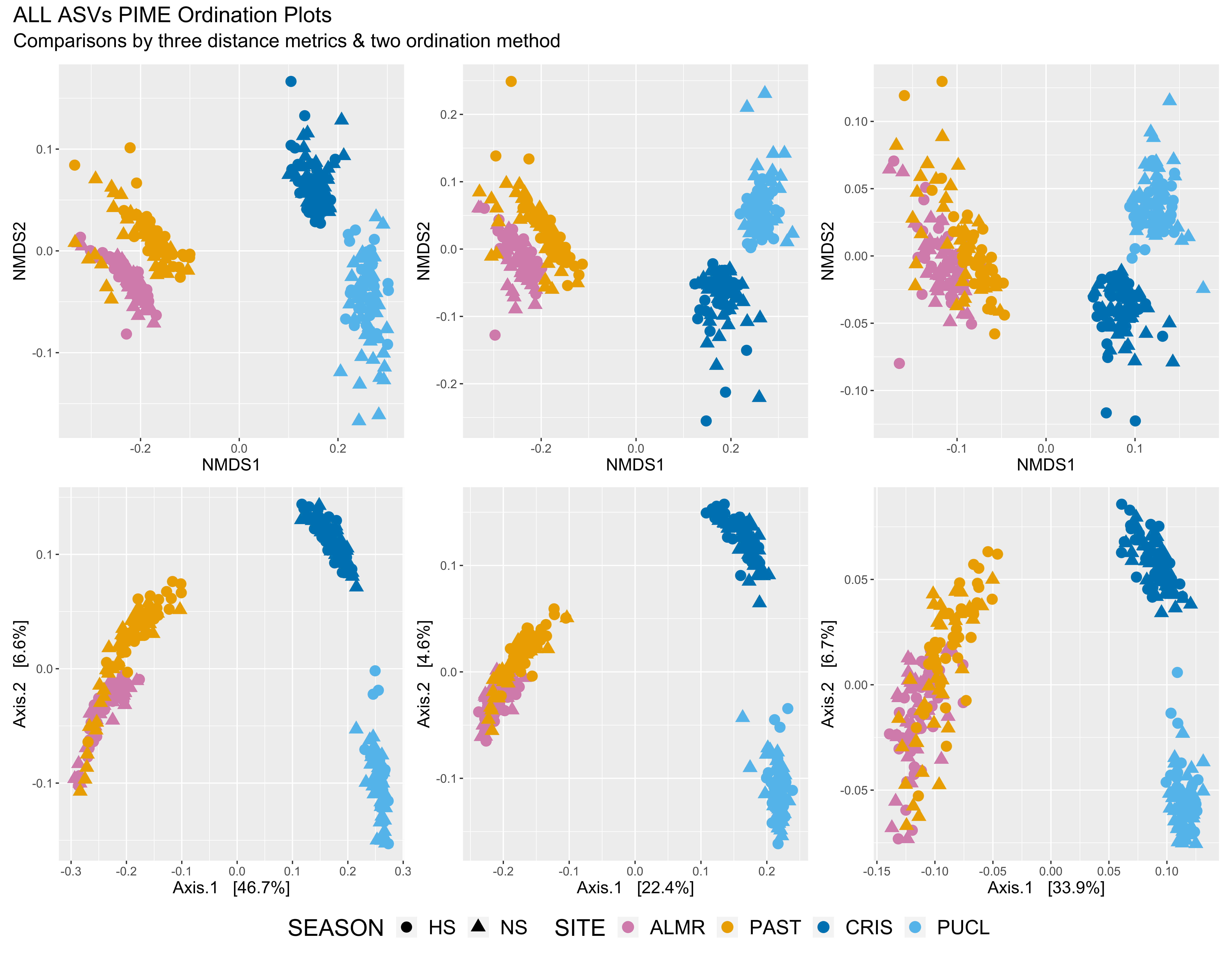
Figure 2: Left = Jensen-Shannon Divergence, middle = UniFrac (unwieghted), right = UniFrac (wieghted); Top = NMDS, bottom = PCoA.
Beta Diversity Plots (by Site)
Here we visualize the different distance matrices using several ordination methods on the ALL and PIME filtered data sets to access dissimilarity among samples from the same site.
Plots ALL ASVs
First, we inspect different ordination methods to see how the samples cluster using weighted-UniFrac, unweighted-UniFrac, and Jensen-Shannon Divergence distance measurements. We could also test different diversity metrics, different transformations, etc.
remove(list = ls())
ssu_ps_work_ALMR <- readRDS("files/trepo/alpha/rdata/ssu_ps_work_ALMR.rds")
ssu_ps_work_CRIS  <- readRDS("files/trepo/alpha/rdata/ssu_ps_work_CRIS.rds")
ssu_ps_work_PAST <- readRDS("files/trepo/alpha/rdata/ssu_ps_work_PAST.rds")
ssu_ps_work_PUCL <- readRDS("files/trepo/alpha/rdata/ssu_ps_work_PUCL.rds")
objects()
Before we begin, we must first transform sample counts to relative abundance for both data sets.
samp_ps <- c("ssu_ps_work_ALMR", "ssu_ps_work_CRIS", "ssu_ps_work_PAST", "ssu_ps_work_PUCL")
for (i in samp_ps) {
     tmp_name <- purrr::map_chr(i, ~ paste0(., "_prop"))
     tmp_get <- get(i)
     tmp_ps <- transform_sample_counts(tmp_get, function(otu) otu/sum(otu))
     tmp_ps@phy_tree <- NULL
     tmp_ps <- prune_samples(sample_sums(tmp_ps) > 0, tmp_ps)
     tmp_tree <- rtree(ntaxa(tmp_ps), rooted = TRUE, tip.label = taxa_names(tmp_ps))
     tmp_ps <- merge_phyloseq(tmp_ps, sample_data, tmp_tree)
     print(tmp_name)
     assign(tmp_name, tmp_ps)
     rm(list = ls(pattern = "tmp_"))
}
samp_ps <- c("ssu_ps_work_ALMR", "ssu_ps_work_CRIS", "ssu_ps_work_PAST", "ssu_ps_work_PUCL")
dist <- c("wunifrac", "unifrac", "jsd")
for (i in samp_ps){
for (d in dist){
tmp_name <- purrr::map_chr(d, ~ paste0(i, "_dist_", .))
tmp_name_plot <- purrr::map_chr(d, ~ paste0(i, "_dist_", ., "_plot"))
tmp_get <- get(purrr::map_chr(i, ~ paste0(., "_prop")))
ord_meths <- c("NMDS", "PCoA", "CCA", "DCA") # MDS = PCoA, "CCA", "DCA", "DPCoA", "RDA"
tmp_plist_name <- purrr::map_chr(d, ~ paste0(i, "_", ., "_plist"))
tmp_plist <- llply(as.list(ord_meths), function(i, physeq, d) {
ordi = ordinate(physeq, method = i, distance = d)
plot_ordination(physeq, ordi, "samples", color = "SEASON")
}, tmp_get, d)
names(tmp_plist) <- ord_meths
tmp_df <- ldply(tmp_plist, function(x){
df = x$data[, 1:2]
colnames(df) = c("Axis_1", "Axis_2")
return(cbind(df, x$data))})
names(tmp_df)[1] = "method"
## NEXT LINE REORDER FACTORS
tmp_df$SITE <- factor(tmp_df$SITE, levels = c("ALMR", "PAST", "CRIS", "PUCL"))
tmp_plot <- ggplot(tmp_df, aes(Axis_1, Axis_2,
color = SEASON, shape = SEASON, fill = SEASON))
tmp_plot <- tmp_plot + geom_point(size = 2)
tmp_plot <- tmp_plot + facet_wrap(~method, scales = "free")
tmp_plot <- tmp_plot + scale_colour_manual(values = swel_col)
assign(tmp_plist_name, tmp_plist)
assign(tmp_name, tmp_df)
assign(tmp_name_plot, tmp_plot)
rm(list = ls(pattern = "tmp_"))
}
}
objects(pattern = "_dist_")
objects()plist_name <- objects(pattern="_plist")
plot_num <- c(1,2)
for (i in plist_name) {
for (j in plot_num) {
tmp_get_i <- get(i)
## NEXT LINE REORDER FACTORS
tmp_get_i[[j]]$data$SITE <- factor(tmp_get_i[[j]]$data$SITE,
levels = c("ALMR", "PAST", "CRIS", "PUCL"))
tmp_ord <- names(tmp_get_i)[j]
tmp_name <- stringr::str_replace(i, "plist", tmp_ord)
tmp_plot <- tmp_get_i[[j]] + scale_colour_manual(values = swel_col)
tmp_plot <- tmp_plot + geom_point(size = 4, aes(shape = SEASON)) +
theme(legend.position = "bottom")
tmp_plot$labels$shape <- "SEASON"
assign(tmp_name, tmp_plot)
rm(list = ls(pattern = "tmp_"))
}
}Almirante (inner bay)
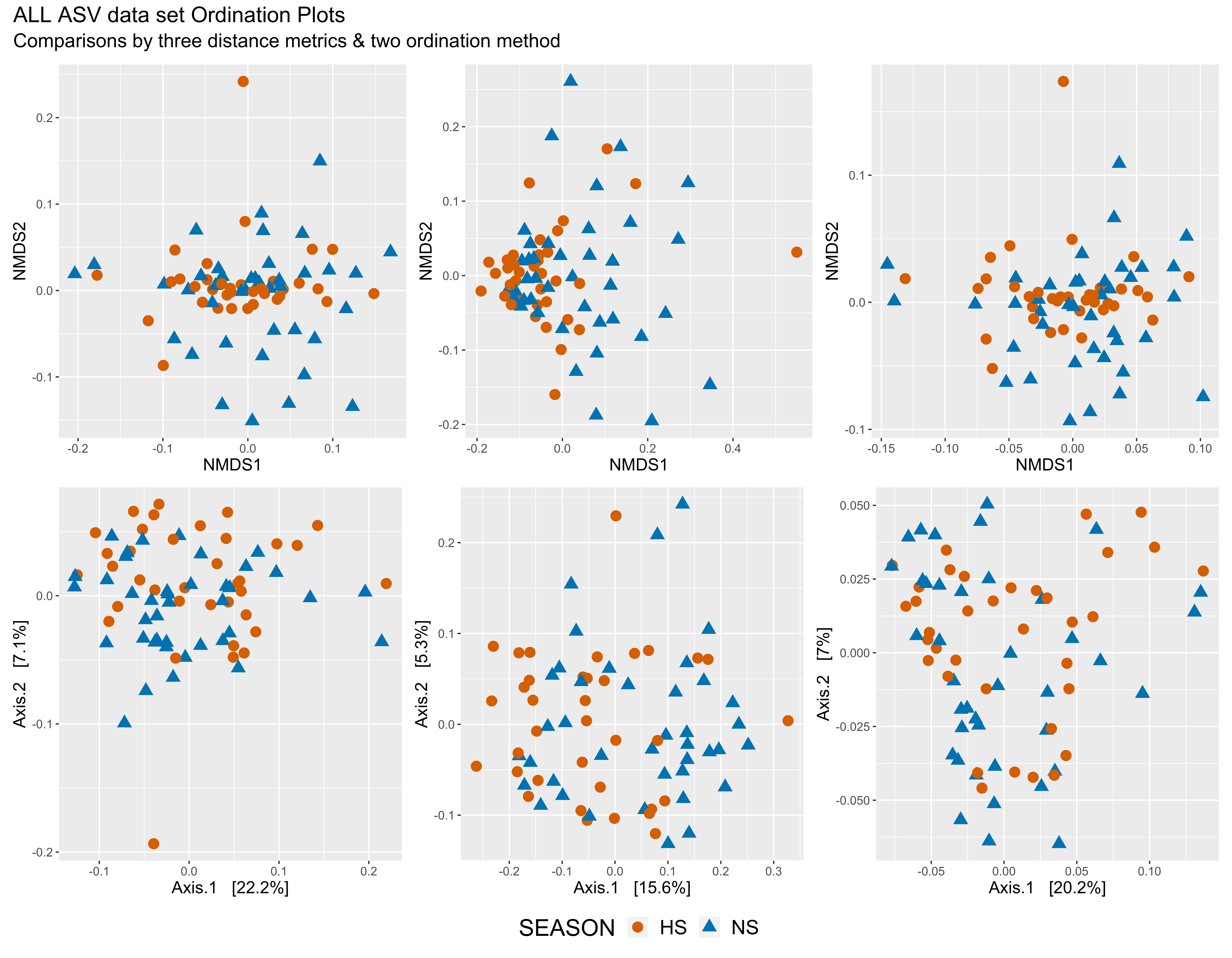
Figure 3: Left = Jensen-Shannon Divergence, middle = UniFrac (unwieghted), right = UniFrac (wieghted); Top = NMDS, bottom = PCoA.
Pastores (inner bay)
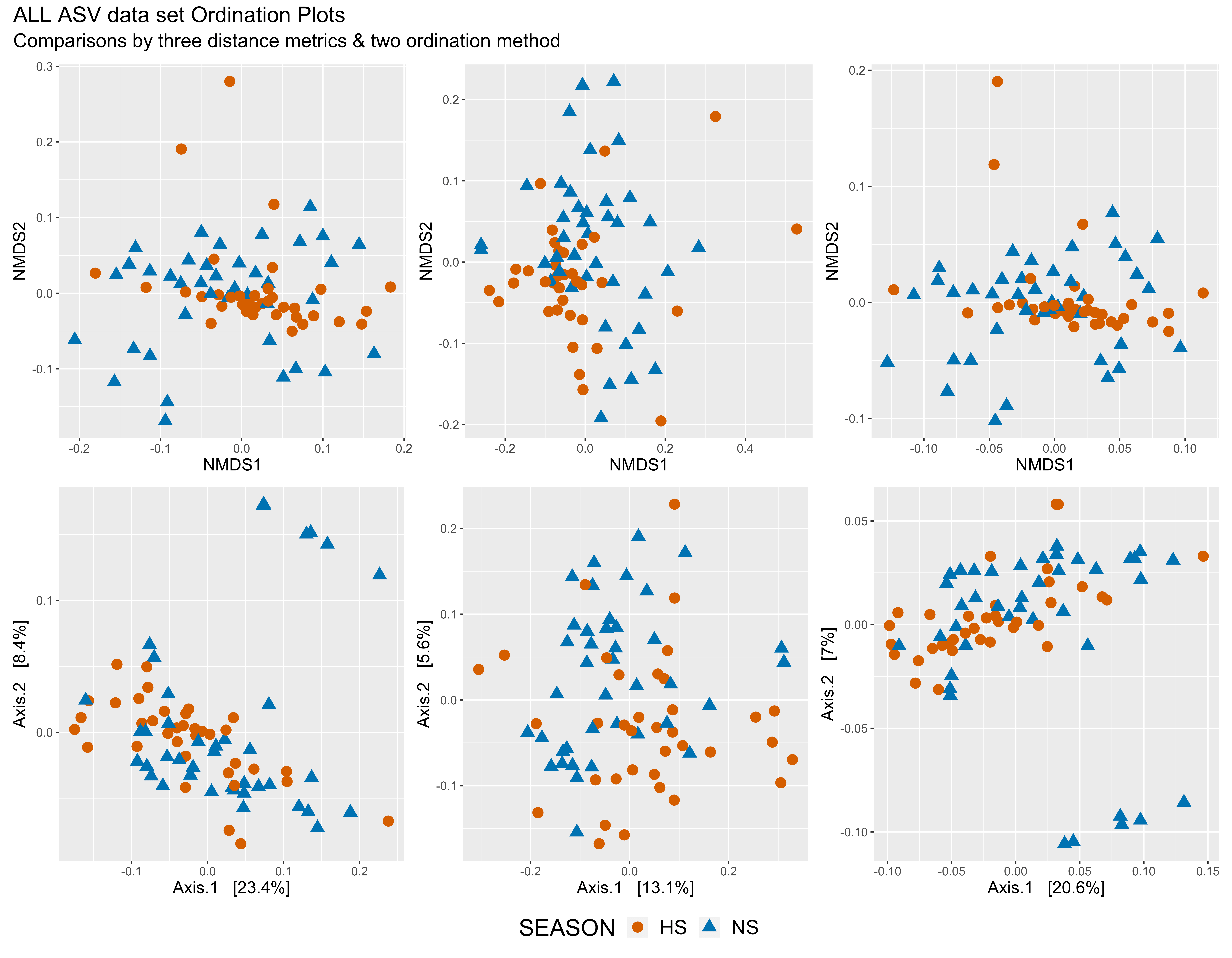
Figure 4: Left = Jensen-Shannon Divergence, middle = UniFrac (unwieghted), right = UniFrac (wieghted); Top = NMDS, bottom = PCoA.
Cristobal (outer bay)
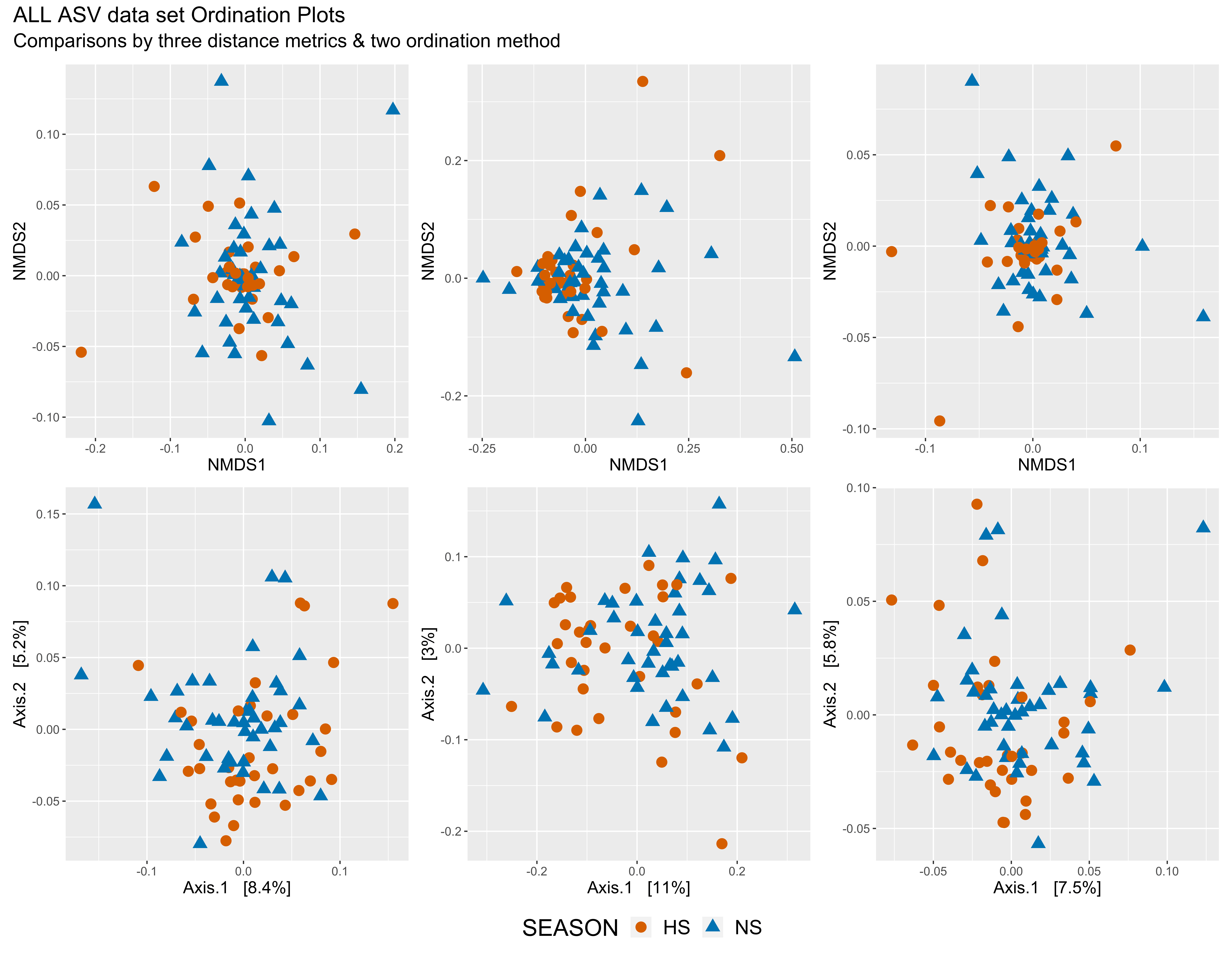
Figure 5: Left = Jensen-Shannon Divergence, middle = UniFrac (unwieghted), right = UniFrac (wieghted); Top = NMDS, bottom = PCoA.
Punta Caracol (outer bay)
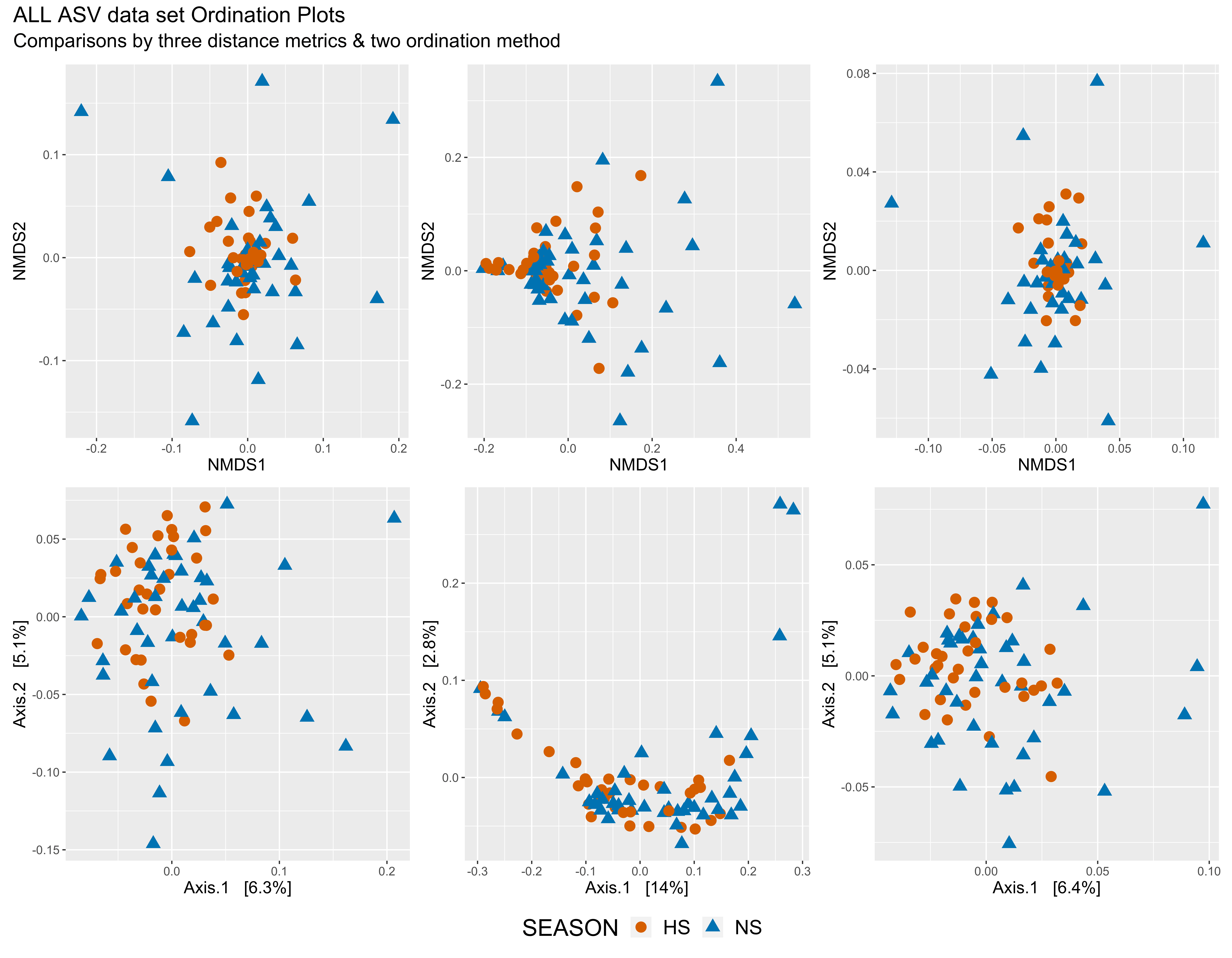
Figure 6: Left = Jensen-Shannon Divergence, middle = UniFrac (unwieghted), right = UniFrac (wieghted); Top = NMDS, bottom = PCoA.
Plots PIME ASVs
remove(list = ls())
ssu_ps_pime_ALMR <- readRDS("files/trepo/pime/rdata/ssu_ps_asv_pime_ALMR.rds")
ssu_ps_pime_CRIS <- readRDS("files/trepo/pime/rdata/ssu_ps_asv_pime_CRIS.rds")
ssu_ps_pime_PAST <- readRDS("files/trepo/pime/rdata/ssu_ps_asv_pime_PAST.rds")
ssu_ps_pime_PUCL <- readRDS("files/trepo/pime/rdata/ssu_ps_asv_pime_PUCL.rds")
objects()Before we begin, we must first transform sample counts to relative abundance for both data sets.
samp_ps <- c("ssu_ps_pime_ALMR", "ssu_ps_pime_CRIS", "ssu_ps_pime_PAST", "ssu_ps_pime_PUCL")
for (i in samp_ps) {
tmp_name <- purrr::map_chr(i, ~ paste0(., "_prop"))
tmp_get <- get(i)
tmp_ps <- transform_sample_counts(tmp_get, function(otu) otu/sum(otu))
tmp_ps@phy_tree <- NULL
tmp_ps <- prune_samples(sample_sums(tmp_ps) > 0, tmp_ps)
tmp_tree <- rtree(ntaxa(tmp_ps), rooted = TRUE, tip.label = taxa_names(tmp_ps))
tmp_ps <- merge_phyloseq(tmp_ps, sample_data, tmp_tree)
print(tmp_name)
assign(tmp_name, tmp_ps)
rm(list = ls(pattern = "tmp_"))
}samp_ps <- c("ssu_ps_pime_ALMR", "ssu_ps_pime_CRIS", "ssu_ps_pime_PAST", "ssu_ps_pime_PUCL")
dist <- c("wunifrac", "unifrac", "jsd")
for (i in samp_ps){
for (d in dist){
tmp_name <- purrr::map_chr(d, ~ paste0(i, "_dist_", .))
tmp_name_plot <- purrr::map_chr(d, ~ paste0(i, "_dist_", ., "_plot"))
tmp_get <- get(purrr::map_chr(i, ~ paste0(., "_prop")))
ord_meths <- c("NMDS", "PCoA", "CCA", "DCA") # MDS = PCoA, "CCA", "DCA", "DPCoA", "RDA"
tmp_plist_name <- purrr::map_chr(d, ~ paste0(i, "_", ., "_plist"))
tmp_plist <- llply(as.list(ord_meths), function(i, physeq, d) {
ordi = ordinate(physeq, method = i, distance = d)
plot_ordination(physeq, ordi, "samples", color = "SEASON")
}, tmp_get, d)
names(tmp_plist) <- ord_meths
tmp_df <- ldply(tmp_plist, function(x){
df = x$data[, 1:2]
colnames(df) = c("Axis_1", "Axis_2")
return(cbind(df, x$data))})
names(tmp_df)[1] = "method"
## NEXT LINE REORDER FACTORS
tmp_df$SITE <- factor(tmp_df$SITE, levels = c("ALMR", "PAST", "CRIS", "PUCL"))
tmp_plot <- ggplot(tmp_df, aes(Axis_1, Axis_2,
color = SEASON, shape = SEASON, fill = SEASON))
tmp_plot <- tmp_plot + geom_point(size = 2)
tmp_plot <- tmp_plot + facet_wrap(~method, scales = "free")
tmp_plot <- tmp_plot + scale_colour_manual(values = swel_col)
assign(tmp_plist_name, tmp_plist)
assign(tmp_name, tmp_df)
assign(tmp_name_plot, tmp_plot)
rm(list = ls(pattern = "tmp_"))
}
}
objects(pattern = "_dist_")
objects()plist_name <- objects(pattern="_plist")
plot_num <- c(1,2)
for (i in plist_name) {
for (j in plot_num) {
tmp_get_i <- get(i)
## NEXT LINE REORDER FACTORS
tmp_get_i[[j]]$data$SITE <- factor(tmp_get_i[[j]]$data$SITE,
levels = c("ALMR", "PAST", "CRIS", "PUCL"))
tmp_ord <- names(tmp_get_i)[j]
tmp_name <- stringr::str_replace(i, "plist", tmp_ord)
tmp_plot <- tmp_get_i[[j]] + scale_colour_manual(values = swel_col)
tmp_plot <- tmp_plot + geom_point(size = 4, aes(shape = SEASON)) +
theme(legend.position = "bottom")
tmp_plot$labels$shape <- "SEASON"
assign(tmp_name, tmp_plot)
rm(list = ls(pattern = "tmp_"))
}
}Almirante (inner bay)
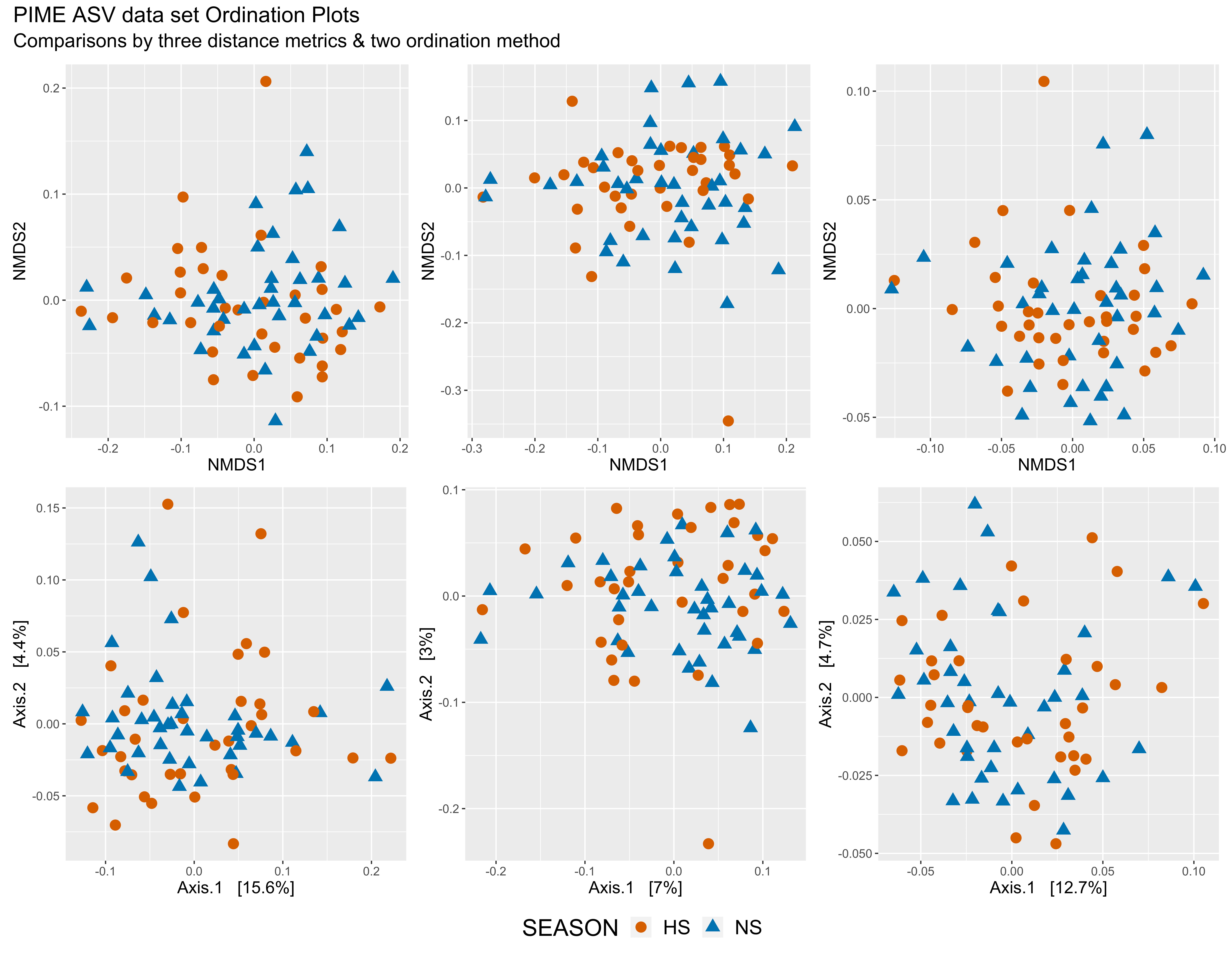
Figure 7: Left = Jensen-Shannon Divergence, middle = UniFrac (unwieghted), right = UniFrac (wieghted); Top = NMDS, bottom = PCoA.
Pastores (inner bay)
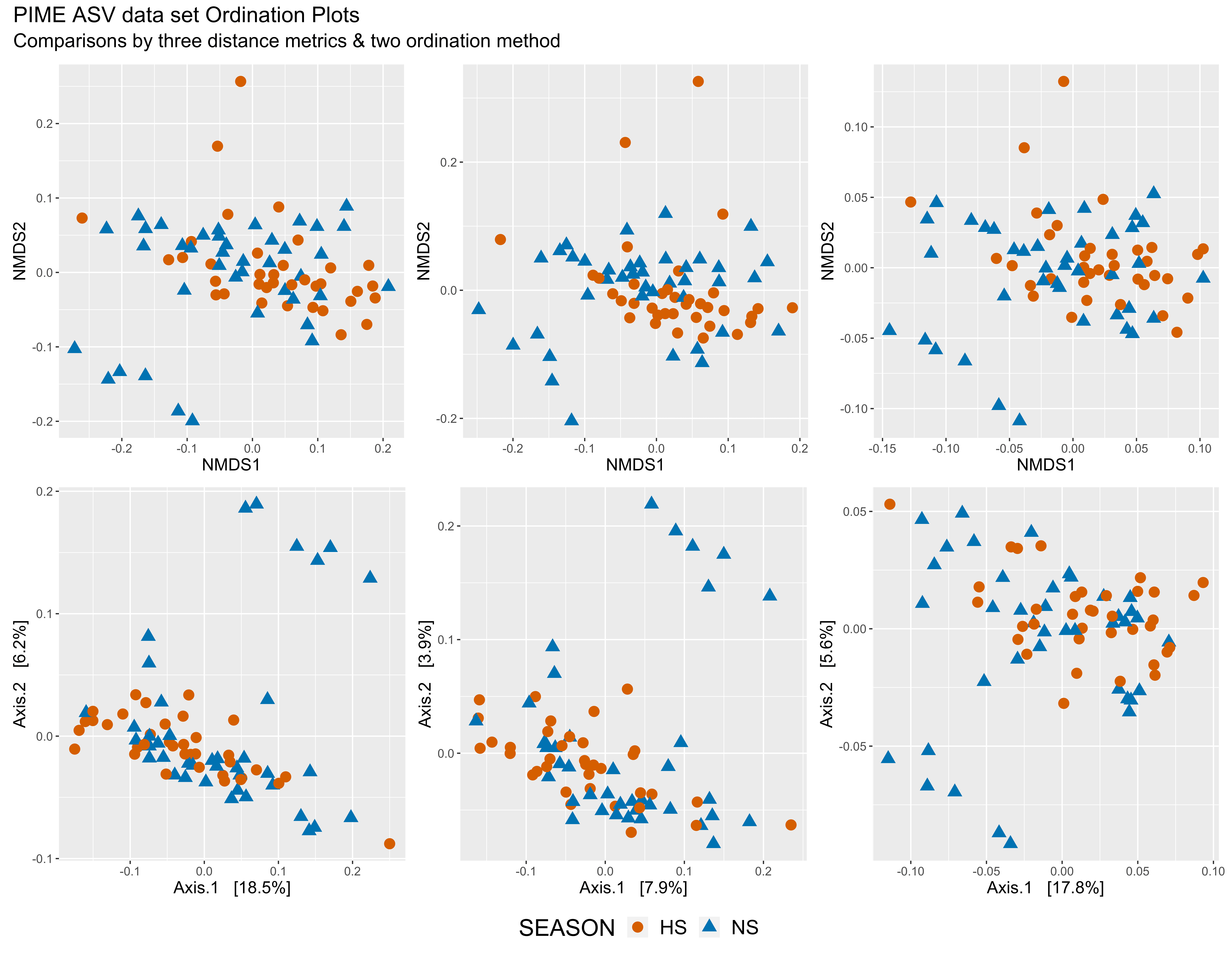
Figure 8: Left = Jensen-Shannon Divergence, middle = UniFrac (unwieghted), right = UniFrac (wieghted); Top = NMDS, bottom = PCoA.
Cristobal (outer bay)
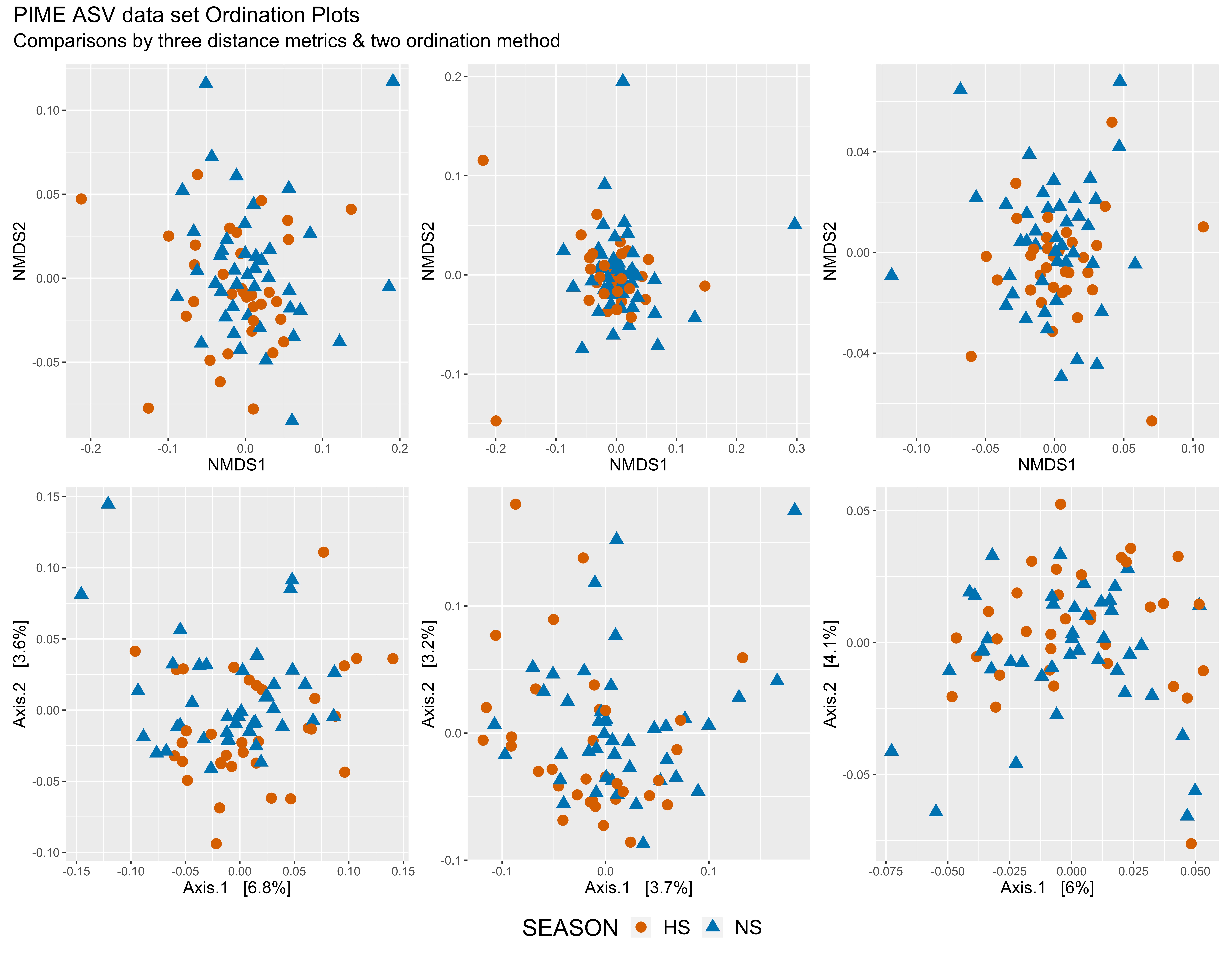
Figure 9: Left = Jensen-Shannon Divergence, middle = UniFrac (unwieghted), right = UniFrac (wieghted); Top = NMDS, bottom = PCoA.
Punta Caracol (outer bay)
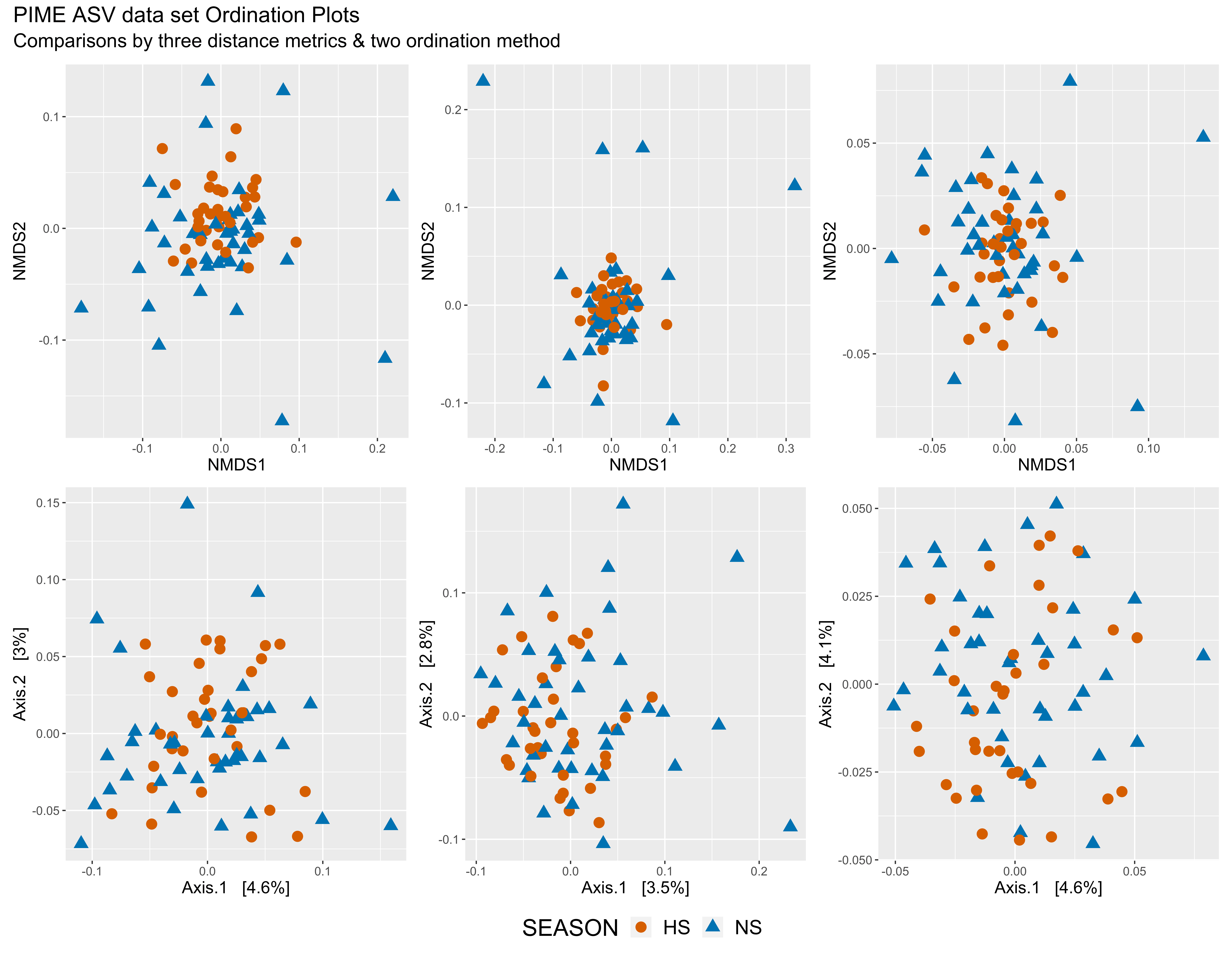
Figure 10: Left = Jensen-Shannon Divergence, middle = UniFrac (unwieghted), right = UniFrac (wieghted); Top = NMDS, bottom = PCoA.
Merged Data Set
Significance Tests
In order to test for significance between sample groups, we must perform the following steps:
- Create distance matrices based on the metrics above (
wunifrac,unifrac,jsd). For this we use the functionphyloseq::distance. - Next, calculate beta dispersion using the
betadisperfunction from theveganpackage. - Then, use the function
permutestto run a Permutation test for homogeneity of multivariate dispersions. - If the beta dispersion tests are not significant we will run a PERMANOVA (since PERMANOVA assumes equal dispersion), otherwise we will use Analysis of Similarity (ANOSIM).
Steps 1, 2, and 3 are analyzed in a for loop that tests all three distance metrics.
Before we begin, we must first transform sample counts to relative abundance for both data sets.
samp_ps <- c("ssu_ps_work", "ssu_ps_pime")
for (i in samp_ps) {
tmp_name <- purrr::map_chr(i, ~ paste0(., "_prop"))
tmp_get <- get(i)
tmp_ps <- transform_sample_counts(tmp_get, function(otu) otu/sum(otu))
tmp_ps@phy_tree <- NULL
tmp_ps <- prune_samples(sample_sums(tmp_ps) > 0, tmp_ps)
tmp_tree <- rtree(ntaxa(tmp_ps), rooted = TRUE, tip.label = taxa_names(tmp_ps))
tmp_ps <- merge_phyloseq(tmp_ps, sample_data, tmp_tree)
print(tmp_name)
assign(tmp_name, tmp_ps)
rm(list = ls(pattern = "tmp_"))
}Beta Dispersion
dist <- c("jsd", "unifrac", "wunifrac")
for (i in samp_ps) {
for (d in dist){
tmp_get <- get(purrr::map_chr(i, ~ paste0(i, "_prop")))
tmp_samp <- data.frame(sample_data(tmp_get))
tmp_df <- phyloseq::distance(tmp_get, method = d)
tmp_df_name <- purrr::map_chr(d, ~ paste0(i, "_beta_dist_", .))
assign(tmp_df_name, tmp_df)
tmp_df2 <- betadisper(tmp_df, tmp_samp$SITE, bias.adjust = TRUE)
tmp_df_name2 <- purrr::map_chr(d, ~ paste0(i, "_beta_dispersion_", .))
assign(tmp_df_name2, tmp_df2)
tmp_df3 <- permutest(tmp_df2, pairwise = TRUE,
permutations = 1000, binary = FALSE)
tmp_df_name3 <- purrr::map_chr(d, ~ paste0(i, "_permutest_", .))
assign(tmp_df_name3, tmp_df3)
rm(list = ls(pattern = "tmp_"))
}
}
objects()Detailed results of Beta Dispersion & Permutation tests
Permutation tests (ASV)
***** ssu_ps_work *****
####################################################
BETA DISPERSION significance test jsd distance
####################################################
Permutation test for homogeneity of multivariate dispersions
Permutation: free
Number of permutations: 1000
Response: Distances
Df Sum Sq Mean Sq F N.Perm Pr(>F)
Groups 3 0.010976 0.0036585 3.4265 1000 0.02098 *
Residuals 100 0.106771 0.0010677
---
Signif. codes: 0 '***' 0.001 '**' 0.01 '*' 0.05 '.' 0.1 ' ' 1
Pairwise comparisons:
(Observed p-value below diagonal, permuted p-value above
diagonal)
ALMR CRIS PAST PUCL
ALMR 0.0039960 0.0089910 0.0140
CRIS 0.0032878 0.7422577 0.9391
PAST 0.0133486 0.7425251 0.8192
PUCL 0.0117791 0.9393926 0.8168891
####################################################
BETA DISPERSION significance test unifrac distance
####################################################
Permutation test for homogeneity of multivariate dispersions
Permutation: free
Number of permutations: 1000
Response: Distances
Df Sum Sq Mean Sq F N.Perm Pr(>F)
Groups 3 0.010562 0.0035206 1.8701 1000 0.1469
Residuals 100 0.188259 0.0018826
Pairwise comparisons:
(Observed p-value below diagonal, permuted p-value above
diagonal)
ALMR CRIS PAST PUCL
ALMR 0.055944 0.089910 0.4126
CRIS 0.046394 0.804196 0.1888
PAST 0.087320 0.824809 0.2987
PUCL 0.427589 0.192537 0.309912
####################################################
BETA DISPERSION significance test wunifrac distance
####################################################
Permutation test for homogeneity of multivariate dispersions
Permutation: free
Number of permutations: 1000
Response: Distances
Df Sum Sq Mean Sq F N.Perm Pr(>F)
Groups 3 0.002711 0.00090379 1.8126 1000 0.1499
Residuals 100 0.049861 0.00049861
Pairwise comparisons:
(Observed p-value below diagonal, permuted p-value above
diagonal)
ALMR CRIS PAST PUCL
ALMR 0.168831 0.058941 0.1908
CRIS 0.158753 0.259740 0.8671
PAST 0.046665 0.270591 0.3936
PUCL 0.176810 0.874601 0.370417
***** ssu_ps_pime *****
####################################################
BETA DISPERSION significance test jsd distance
####################################################
Permutation test for homogeneity of multivariate dispersions
Permutation: free
Number of permutations: 1000
Response: Distances
Df Sum Sq Mean Sq F N.Perm Pr(>F)
Groups 3 0.005337 0.00177907 4.6404 1000 0.004995 **
Residuals 100 0.038339 0.00038339
---
Signif. codes: 0 '***' 0.001 '**' 0.01 '*' 0.05 '.' 0.1 ' ' 1
Pairwise comparisons:
(Observed p-value below diagonal, permuted p-value above
diagonal)
ALMR CRIS PAST PUCL
ALMR 0.14285714 0.00499500 0.0010
CRIS 0.13505721 0.07692308 0.0200
PAST 0.00966154 0.06683560 0.6953
PUCL 0.00077929 0.01979019 0.68542506
####################################################
BETA DISPERSION significance test unifrac distance
####################################################
Permutation test for homogeneity of multivariate dispersions
Permutation: free
Number of permutations: 1000
Response: Distances
Df Sum Sq Mean Sq F N.Perm Pr(>F)
Groups 3 0.002844 0.00094792 1.7709 1000 0.1598
Residuals 100 0.053527 0.00053527
Pairwise comparisons:
(Observed p-value below diagonal, permuted p-value above
diagonal)
ALMR CRIS PAST PUCL
ALMR 0.336663 0.089910 0.8032
CRIS 0.331774 0.345654 0.2168
PAST 0.096959 0.368463 0.0539
PUCL 0.788697 0.208651 0.056996
####################################################
BETA DISPERSION significance test wunifrac distance
####################################################
Permutation test for homogeneity of multivariate dispersions
Permutation: free
Number of permutations: 1000
Response: Distances
Df Sum Sq Mean Sq F N.Perm Pr(>F)
Groups 3 0.0014351 0.00047837 3.0034 1000 0.03596 *
Residuals 100 0.0159274 0.00015927
---
Signif. codes: 0 '***' 0.001 '**' 0.01 '*' 0.05 '.' 0.1 ' ' 1
Pairwise comparisons:
(Observed p-value below diagonal, permuted p-value above
diagonal)
ALMR CRIS PAST PUCL
ALMR 0.852148 0.038961 0.1838
CRIS 0.844035 0.049950 0.1668
PAST 0.042375 0.039063 0.1888
PUCL 0.182975 0.146451 0.185432 Remember, if the beta dispersion p-value is greater than 0.05 we use PERMANOVA, otherwise we use ANOSIM.
file.remove("files/trepo/beta/tables/tmp_merge.txt")
for (i in samp_ps) {
for (d in dist){
tmp_get <- get(purrr::map_chr(i, ~ paste0(., "_permutest_", d)))
tmp_res <- eval(isTRUE(tmp_get$tab$`Pr(>F)`[1] < 0.05))
tmp_print <- c("Permutation test p-value of ", i, d,
" < 0.05?", tmp_res)
cat(tmp_print,"\n", append = TRUE, file = "files/trepo/beta/tables/tmp_merge.txt")
rm(list = ls(pattern = "tmp_"))
}
}
ssu_perm_pvalues <- read_delim("files/trepo/beta/tables/tmp_merge.txt", delim = "\n", col_names = "permutation results")Significance Tests (ALL ASVs)
# A tibble: 3 x 1
`permutation results`
<chr>
1 "Permutation test p-value of ssu_ps_work jsd < 0.05? TRUE "
2 "Permutation test p-value of ssu_ps_work unifrac < 0.05? FALSE "
3 "Permutation test p-value of ssu_ps_work wunifrac < 0.05? FALSE "ssu_ps_work_adonis_jsd <- adonis(ssu_ps_work_beta_dist_jsd ~ SITE,
data = adonis_sampledf, permutations = 1000)
ssu_ps_work_adonis2_jsd <- adonis2(ssu_ps_work_beta_dist_jsd ~ SITE,
data = adonis_sampledf, permutations = 1000)ssu_ps_work_groups <- get_variable(anosim_data, "SITE")
ssu_ps_work_anosim_unifrac <-
anosim(phyloseq::distance(ssu_ps_work_prop, "unifrac"),
grouping = ssu_ps_work_groups)ssu_ps_work_groups <- get_variable(anosim_data, "SITE")
ssu_ps_work_anosim_wunifrac <-
anosim(phyloseq::distance(ssu_ps_work_prop, "wunifrac"),
grouping = ssu_ps_work_groups)Detailed results of Significance tests for the ALL ASV data set
***PERMANOVA for Jensen-Shannon Divergence, `jsd`*** Permutation test for adonis under reduced model
Terms added sequentially (first to last)
Permutation: free
Number of permutations: 1000
adonis2(formula = ssu_ps_work_beta_dist_jsd ~ SITE, data = adonis_sampledf, permutations = 1000)
Df SumOfSqs R2 F Pr(>F)
SITE 3 5.3763 0.81399 145.87 0.000999 ***
Residual 100 1.2286 0.18601
Total 103 6.6049 1.00000
---
Signif. codes: 0 '***' 0.001 '**' 0.01 '*' 0.05 '.' 0.1 ' ' 1
***ANOSIM for Unweighted UniFrac distance, `unifrac`***
Call:
anosim(x = phyloseq::distance(ssu_ps_work_prop, "unifrac"), grouping = ssu_ps_work_groups)
Dissimilarity:
ANOSIM statistic R: 0.8123
Significance: 0.001
Permutation: free
Number of permutations: 999
Upper quantiles of permutations (null model):
90% 95% 97.5% 99%
0.0235 0.0321 0.0419 0.0543
Dissimilarity ranks between and within classes:
0% 25% 50% 75% 100% N
Between 7 2219.75 3326.5 4342.25 5356 4056
ALMR 5 121.00 636.0 1285.00 3385 325
CRIS 91 804.00 1165.0 1517.00 3533 325
PAST 2 567.00 1095.0 1678.00 3113 325
PUCL 1 383.00 751.0 1422.00 3149 325
***ANOSIM for Weighted-UniFrac distance, `wunifrac`***
Call:
anosim(x = phyloseq::distance(ssu_ps_work_prop, "wunifrac"), grouping = ssu_ps_work_groups)
Dissimilarity:
ANOSIM statistic R: 0.9244
Significance: 0.001
Permutation: free
Number of permutations: 999
Upper quantiles of permutations (null model):
90% 95% 97.5% 99%
0.0231 0.0343 0.0456 0.0622
Dissimilarity ranks between and within classes:
0% 25% 50% 75% 100% N
Between 324 2290.75 3328.5 4342.25 5356 4056
ALMR 1 174.00 387.0 844.00 2253 325
CRIS 48 442.00 701.0 977.00 2080 325
PAST 5 415.00 875.0 1646.00 2707 325
PUCL 3 405.00 794.0 1272.00 1988 325Significance Tests (PIME ASVs)
# A tibble: 3 x 1
`permutation results`
<chr>
1 "Permutation test p-value of ssu_ps_pime jsd < 0.05? TRUE "
2 "Permutation test p-value of ssu_ps_pime unifrac < 0.05? FALSE "
3 "Permutation test p-value of ssu_ps_pime wunifrac < 0.05? TRUE "ssu_ps_pime_adonis_jsd <- adonis(ssu_ps_pime_beta_dist_jsd ~ SITE,
data = adonis_sampledf, permutations = 1000)
ssu_ps_pime_adonis2_jsd <- adonis2(ssu_ps_pime_beta_dist_jsd ~ SITE,
data = adonis_sampledf, permutations = 1000)ssu_ps_pime_groups <- get_variable(anosim_data, "SITE")
ssu_ps_pime_anosim_unifrac <-
anosim(phyloseq::distance(ssu_ps_pime_prop, "unifrac"),
grouping = ssu_ps_pime_groups)ssu_ps_pime_groups <- get_variable(anosim_data, "SITE")
ssu_ps_pime_anosim_wunifrac <-
anosim(phyloseq::distance(ssu_ps_pime_prop, "wunifrac"),
grouping = ssu_ps_pime_groups)Detailed results of Significance tests for PIME data set
***PERMANOVA for Jensen-Shannon Divergence, `jsd`*** Permutation test for adonis under reduced model
Terms added sequentially (first to last)
Permutation: free
Number of permutations: 1000
adonis2(formula = ssu_ps_pime_beta_dist_jsd ~ SITE, data = adonis_sampledf, permutations = 1000)
Df SumOfSqs R2 F Pr(>F)
SITE 3 5.8218 0.807 139.38 0.000999 ***
Residual 100 1.3924 0.193
Total 103 7.2141 1.000
---
Signif. codes: 0 '***' 0.001 '**' 0.01 '*' 0.05 '.' 0.1 ' ' 1
***ANOSIM for Unweighted UniFrac distance, `unifrac`***
Call:
anosim(x = phyloseq::distance(ssu_ps_pime_prop, "unifrac"), grouping = ssu_ps_pime_groups)
Dissimilarity:
ANOSIM statistic R: 0.9769
Significance: 0.001
Permutation: free
Number of permutations: 999
Upper quantiles of permutations (null model):
90% 95% 97.5% 99%
0.0216 0.0324 0.0440 0.0547
Dissimilarity ranks between and within classes:
0% 25% 50% 75% 100% N
Between 888 2314.75 3328.5 4342.25 5356 4056
ALMR 13 205.00 528.0 894.00 1940 325
CRIS 14 468.00 714.0 964.00 1894 325
PAST 22 471.00 879.0 1210.00 2178 325
PUCL 1 264.00 495.0 818.00 1662 325
***ANOSIM for Weighted-UniFrac distance, `wunifrac`***
Call:
anosim(x = phyloseq::distance(ssu_ps_pime_prop, "wunifrac"), grouping = ssu_ps_pime_groups)
Dissimilarity:
ANOSIM statistic R: 0.9512
Significance: 0.001
Permutation: free
Number of permutations: 999
Upper quantiles of permutations (null model):
90% 95% 97.5% 99%
0.0222 0.0321 0.0419 0.0509
Dissimilarity ranks between and within classes:
0% 25% 50% 75% 100% N
Between 513 2294.5 3328.5 4342.25 5356 4056
ALMR 1 140.0 459.0 879.00 2161 325
CRIS 2 330.0 563.0 810.00 1620 325
PAST 10 366.0 869.0 1606.00 2782 325
PUCL 46 505.0 793.0 1033.00 1764 325Summary
Here is a quick summary of significance tests for the FULL and PIME ASV data sets against the three distance matrices.
| distance metric | p-value (MERGE) | p-value (PIME) |
|---|---|---|
| Jensen-Shannon Divergence | 0.000999 | 0.000999 |
| unweighted UniFrac | 0.001000 | 0.001000 |
| weighted UniFrac | 0.001000 | 0.001000 |
Summary of significant tests for the ALL ASVs and PIME ASVs data sets.
Beta Diversity Plots
Here we visualize the different distance matrices using several ordination methods on the ALL and PIME filtered data sets to access dissimilarity among sample.
Plots ALL ASVs
First, we inspect different ordination methods to see how the samples cluster using weighted-UniFrac, unweighted-UniFrac, and Jensen-Shannon Divergence distance measurements. We could also test different diversity metrics, different transformations, etc.
samp_ps <- "ssu_ps_work"
dist <- c("wunifrac", "unifrac", "jsd")
for (d in dist){
tmp_name <- purrr::map_chr(d, ~ paste0(samp_ps, "_dist_", .))
tmp_name_plot <- purrr::map_chr(d, ~ paste0(samp_ps, "_dist_", ., "_plot"))
tmp_get <- get(purrr::map_chr(samp_ps, ~ paste0(., "_prop")))
ord_meths <- c("NMDS", "PCoA", "CCA", "DCA") # MDS = PCoA, "CCA", "DCA", "DPCoA", "RDA"
tmp_plist_name <- purrr::map_chr(d, ~ paste0(samp_ps, "_", ., "_plist"))
tmp_plist <- llply(as.list(ord_meths), function(i, physeq, d) {
ordi = ordinate(physeq, method = i, distance = d)
plot_ordination(physeq, ordi, "samples", color = "SITE")
}, tmp_get, d)
names(tmp_plist) <- ord_meths
tmp_df <- ldply(tmp_plist, function(x){
df = x$data[, 1:2]
colnames(df) = c("Axis_1", "Axis_2")
return(cbind(df, x$data))})
names(tmp_df)[1] = "method"
## NEXT LINE REORDER FACTORS
tmp_df$SITE <- factor(tmp_df$SITE, levels = c("ALMR", "PAST", "CRIS", "PUCL"))
tmp_plot <- ggplot(tmp_df, aes(Axis_1, Axis_2,
color = SITE, shape = SEASON, fill = SITE))
tmp_plot <- tmp_plot + geom_point(size = 2)
tmp_plot <- tmp_plot + facet_wrap(~method, scales = "free")
tmp_plot <- tmp_plot + scale_colour_manual(values = swel_col)
assign(tmp_plist_name, tmp_plist)
assign(tmp_name, tmp_df)
assign(tmp_name_plot, tmp_plot)
rm(list = ls(pattern = "tmp_"))
}
objects(pattern = "_dist_")
objects()samp_ps <- "ssu_ps_work"
plist_name <- objects(pattern="_plist")
plot_num <- c(1,2)
for (i in plist_name) {
  for (j in plot_num) {
       tmp_get_i <- get(i)
     ## NEXT  LINE REORDER FACTORS
       tmp_get_i[[j]]$data$SITE <- factor(tmp_get_i[[j]]$data$SITE,
                                          levels = c("ALMR", "PAST", "CRIS", "PUCL"))
       tmp_ord <- names(tmp_get_i)[j]
       tmp_name <- stringr::str_replace(i, "plist", tmp_ord)
       tmp_plot <- tmp_get_i[[j]] + scale_colour_manual(values = swel_col)
       tmp_plot <- tmp_plot + geom_point(size = 4, aes(shape = SEASON)) +
         theme(legend.position = "bottom")
       tmp_plot$labels$shape <- "SEASON"
       assign(tmp_name, tmp_plot)
       rm(list = ls(pattern = "tmp_"))
  }
}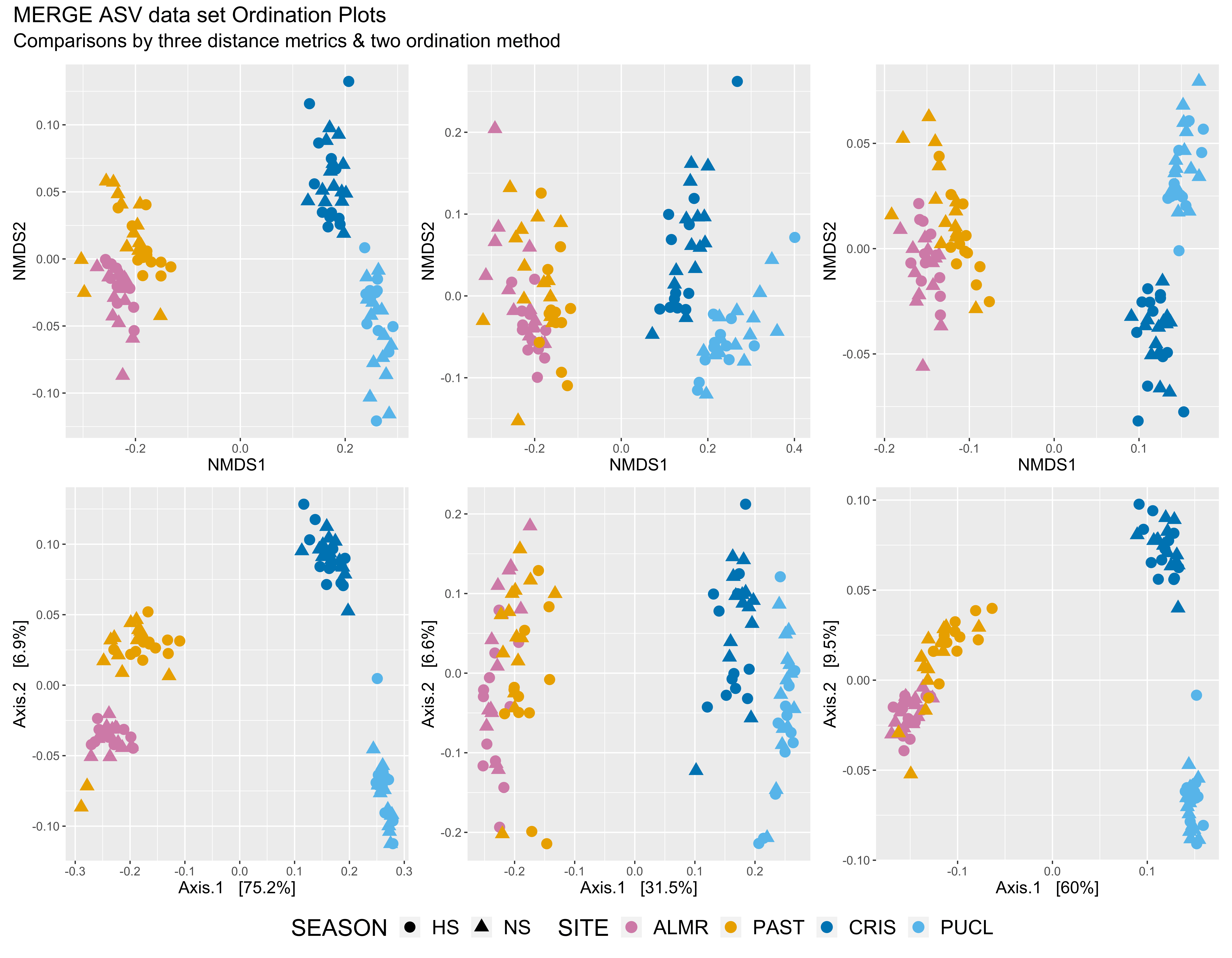
Figure 11: Left = Jensen-Shannon Divergence, middle = UniFrac (unwieghted), right = UniFrac (wieghted); Top = NMDS, bottom = PCoA.
Plots ALL PIME ASV
Same as above, we inspect different ordination methods to see how the samples cluster using weighted-UniFrac, unweighted-UniFrac, and Jensen-Shannon Divergence distance measurements.
samp_ps <- "ssu_ps_pime"
dist <- c("wunifrac", "unifrac", "jsd")
for (d in dist){
tmp_name <- purrr::map_chr(d, ~ paste0(samp_ps, "_dist_", .))
tmp_name_plot <- purrr::map_chr(d, ~ paste0(samp_ps, "_dist_", ., "_plot"))
tmp_get <- get(purrr::map_chr(samp_ps, ~ paste0(., "_prop")))
ord_meths <- c("NMDS", "PCoA", "CCA", "DCA") # MDS = PCoA, "CCA", "DCA", "DPCoA", "RDA"
tmp_plist_name <- purrr::map_chr(d, ~ paste0(samp_ps, "_", ., "_plist"))
tmp_plist <- llply(as.list(ord_meths), function(i, physeq, d) {
ordi = ordinate(physeq, method = i, distance = d)
plot_ordination(physeq, ordi, "samples", color = "SITE")
}, tmp_get, d)
names(tmp_plist) <- ord_meths
tmp_df <- ldply(tmp_plist, function(x){
df = x$data[, 1:2]
colnames(df) = c("Axis_1", "Axis_2")
return(cbind(df, x$data))})
names(tmp_df)[1] = "method"
## NEXT LINE REORDER FACTORS
tmp_df$SITE <- factor(tmp_df$SITE, levels = c("ALMR", "PAST", "CRIS", "PUCL"))
tmp_plot <- ggplot(tmp_df, aes(Axis_1, Axis_2,
color = SITE, shape = SEASON, fill = SITE))
tmp_plot <- tmp_plot + geom_point(size = 2)
tmp_plot <- tmp_plot + facet_wrap(~method, scales = "free")
tmp_plot <- tmp_plot + scale_colour_manual(values = swel_col)
assign(tmp_plist_name, tmp_plist)
assign(tmp_name, tmp_df)
assign(tmp_name_plot, tmp_plot)
rm(list = ls(pattern = "tmp_"))
}samp_ps <- "ssu_ps_pime"
plist_name <- objects(pattern="_plist")
plot_num <- c(1,2)
for (i in plist_name) {
  for (j in plot_num) {
       tmp_get_i <- get(i)
     ## NEXT  LINE REORDER FACTORS
       tmp_get_i[[j]]$data$SITE <- factor(tmp_get_i[[j]]$data$SITE,
                                          levels = c("ALMR", "PAST", "CRIS", "PUCL"))
       tmp_ord <- names(tmp_get_i)[j]
       tmp_name <- stringr::str_replace(i, "plist", tmp_ord)
       tmp_plot <- tmp_get_i[[j]] + scale_colour_manual(values = swel_col)
       tmp_plot <- tmp_plot + geom_point(size = 4, aes(shape = SEASON)) +
         theme(legend.position = "bottom")
       tmp_plot$labels$shape <- "SEASON"
       assign(tmp_name, tmp_plot)
       rm(list = ls(pattern = "tmp_"))
  }
}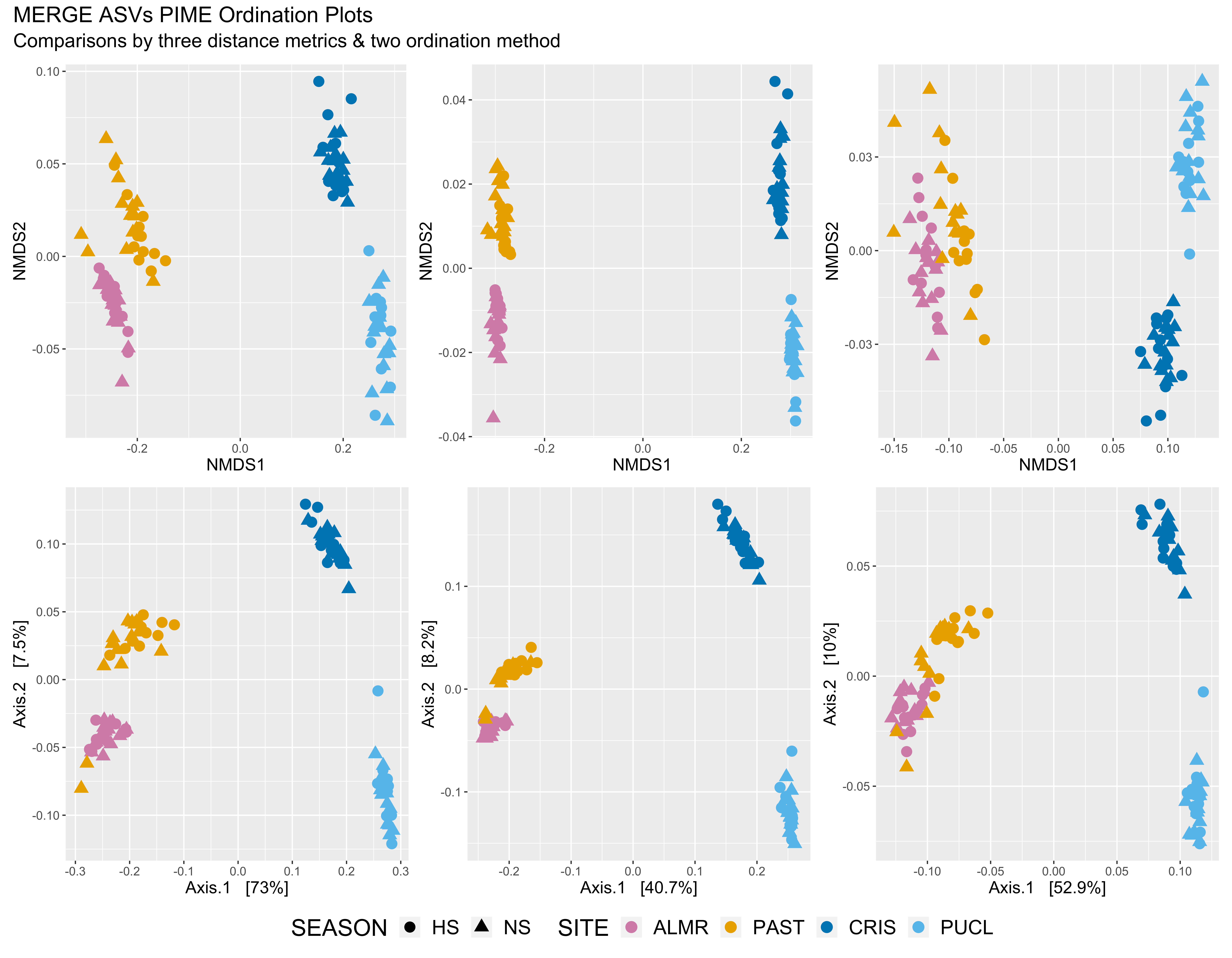
Figure 12: Left = Jensen-Shannon Divergence, middle = UniFrac (unwieghted), right = UniFrac (wieghted); Top = NMDS, bottom = PCoA.
Beta Diversity Plots (by Site)
Here we visualize the different distance matrices using several ordination methods on the ALL and PIME filtered data sets to access dissimilarity among samples from the same site.
Plots ALL ASVs
First, we inspect different ordination methods to see how the samples cluster using weighted-UniFrac, unweighted-UniFrac, and Jensen-Shannon Divergence distance measurements. We could also test different diversity metrics, different transformations, etc.
remove(list = ls())
ssu_ps_work_merge_ALMR <- readRDS("files/trepo/alpha/rdata/ssu_ps_work_merge_ALMR.rds")
ssu_ps_work_merge_CRIS  <- readRDS("files/trepo/alpha/rdata/ssu_ps_work_merge_CRIS.rds")
ssu_ps_work_merge_PAST <- readRDS("files/trepo/alpha/rdata/ssu_ps_work_merge_PAST.rds")
ssu_ps_work_merge_PUCL <- readRDS("files/trepo/alpha/rdata/ssu_ps_work_merge_PUCL.rds")
objects()
Before we begin, we must first transform sample counts to relative abundance for both data sets.
samp_ps <- c("ssu_ps_work_merge_ALMR", "ssu_ps_work_merge_CRIS", "ssu_ps_work_merge_PAST", "ssu_ps_work_merge_PUCL")
for (i in samp_ps) {
     tmp_name <- purrr::map_chr(i, ~ paste0(., "_prop"))
     tmp_get <- get(i)
     tmp_ps <- transform_sample_counts(tmp_get, function(otu) otu/sum(otu))
     tmp_ps@phy_tree <- NULL
     tmp_ps <- prune_samples(sample_sums(tmp_ps) > 0, tmp_ps)
     tmp_tree <- rtree(ntaxa(tmp_ps), rooted = TRUE, tip.label = taxa_names(tmp_ps))
     tmp_ps <- merge_phyloseq(tmp_ps, sample_data, tmp_tree)
     print(tmp_name)
     assign(tmp_name, tmp_ps)
     rm(list = ls(pattern = "tmp_"))
}
samp_ps <- c("ssu_ps_work_merge_ALMR", "ssu_ps_work_merge_CRIS", "ssu_ps_work_merge_PAST", "ssu_ps_work_merge_PUCL")
dist <- c("wunifrac", "unifrac", "jsd")
for (i in samp_ps){
for (d in dist){
tmp_name <- purrr::map_chr(d, ~ paste0(i, "_dist_", .))
tmp_name_plot <- purrr::map_chr(d, ~ paste0(i, "_dist_", ., "_plot"))
tmp_get <- get(purrr::map_chr(i, ~ paste0(., "_prop")))
ord_meths <- c("NMDS", "PCoA", "CCA", "DCA") # MDS = PCoA, "CCA", "DCA", "DPCoA", "RDA"
tmp_plist_name <- purrr::map_chr(d, ~ paste0(i, "_", ., "_plist"))
tmp_plist <- llply(as.list(ord_meths), function(i, physeq, d) {
ordi = ordinate(physeq, method = i, distance = d)
plot_ordination(physeq, ordi, "samples", color = "SEASON")
}, tmp_get, d)
names(tmp_plist) <- ord_meths
tmp_df <- ldply(tmp_plist, function(x){
df = x$data[, 1:2]
colnames(df) = c("Axis_1", "Axis_2")
return(cbind(df, x$data))})
names(tmp_df)[1] = "method"
## NEXT LINE REORDER FACTORS
tmp_df$SITE <- factor(tmp_df$SITE, levels = c("ALMR", "PAST", "CRIS", "PUCL"))
tmp_plot <- ggplot(tmp_df, aes(Axis_1, Axis_2,
color = SEASON, shape = SEASON, fill = SEASON))
tmp_plot <- tmp_plot + geom_point(size = 2)
tmp_plot <- tmp_plot + facet_wrap(~method, scales = "free")
tmp_plot <- tmp_plot + scale_colour_manual(values = swel_col)
assign(tmp_plist_name, tmp_plist)
assign(tmp_name, tmp_df)
assign(tmp_name_plot, tmp_plot)
rm(list = ls(pattern = "tmp_"))
}
}
objects(pattern = "_dist_")
objects()plist_name <- objects(pattern="_plist")
plot_num <- c(1,2)
for (i in plist_name) {
for (j in plot_num) {
tmp_get_i <- get(i)
## NEXT LINE REORDER FACTORS
tmp_get_i[[j]]$data$SITE <- factor(tmp_get_i[[j]]$data$SITE,
levels = c("ALMR", "PAST", "CRIS", "PUCL"))
tmp_ord <- names(tmp_get_i)[j]
tmp_name <- stringr::str_replace(i, "plist", tmp_ord)
tmp_plot <- tmp_get_i[[j]] + scale_colour_manual(values = swel_col)
tmp_plot <- tmp_plot + geom_point(size = 4, aes(shape = SEASON)) +
theme(legend.position = "bottom")
tmp_plot$labels$shape <- "SEASON"
assign(tmp_name, tmp_plot)
rm(list = ls(pattern = "tmp_"))
}
}Almirante (inner bay)
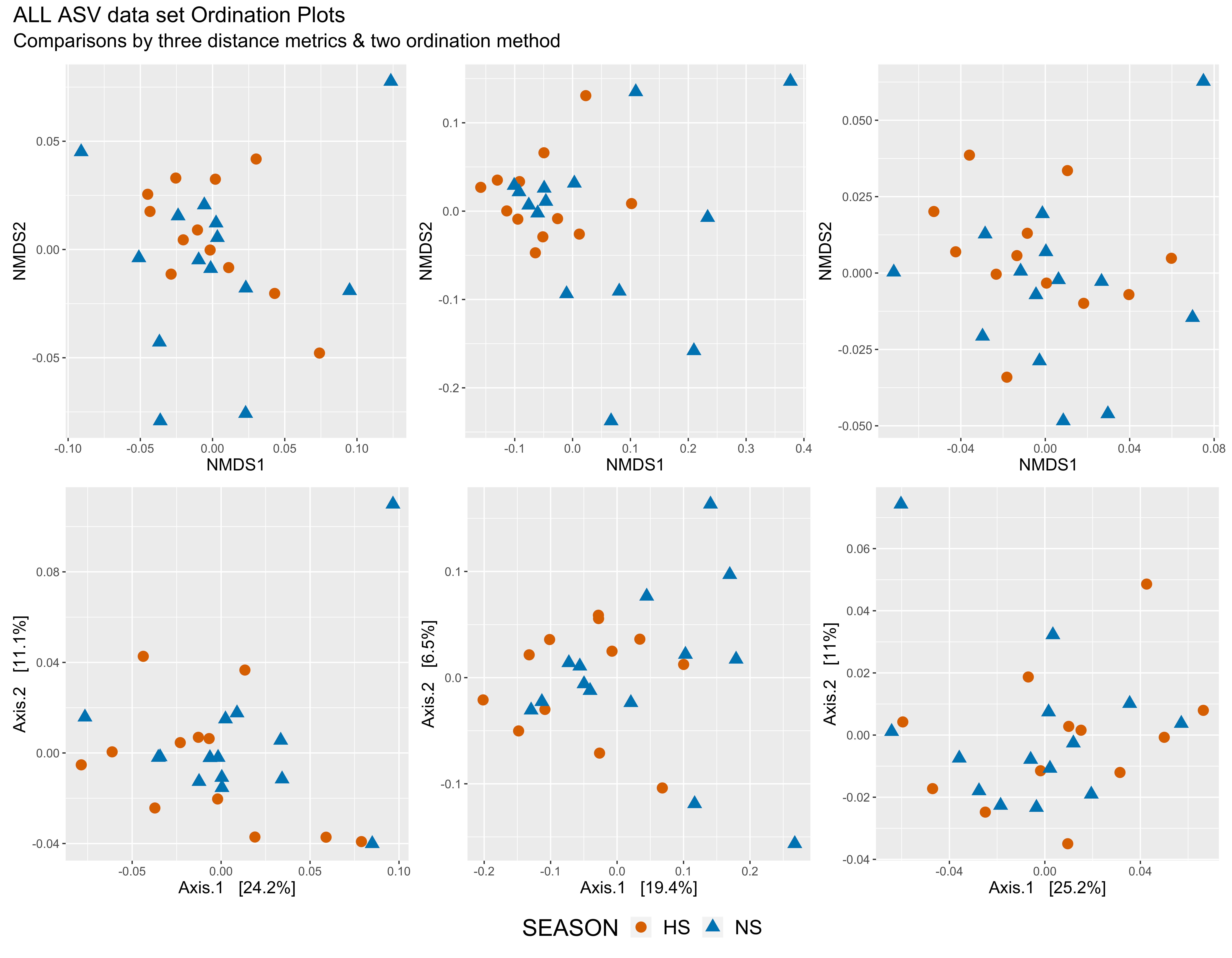
Figure 13: Left = Jensen-Shannon Divergence, middle = UniFrac (unwieghted), right = UniFrac (wieghted); Top = NMDS, bottom = PCoA.
Pastores (inner bay)
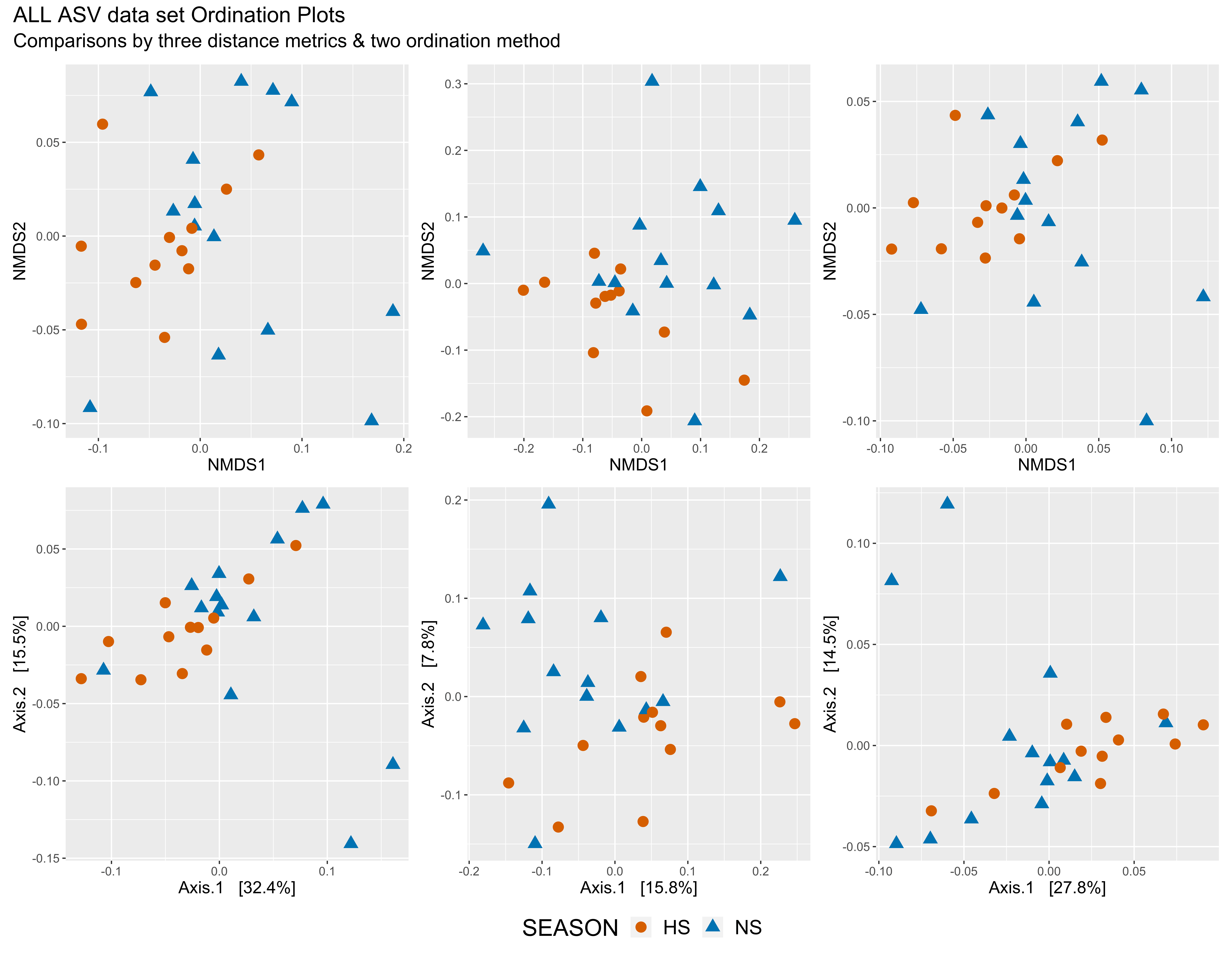
Figure 14: Left = Jensen-Shannon Divergence, middle = UniFrac (unwieghted), right = UniFrac (wieghted); Top = NMDS, bottom = PCoA.
Cristobal (outer bay)
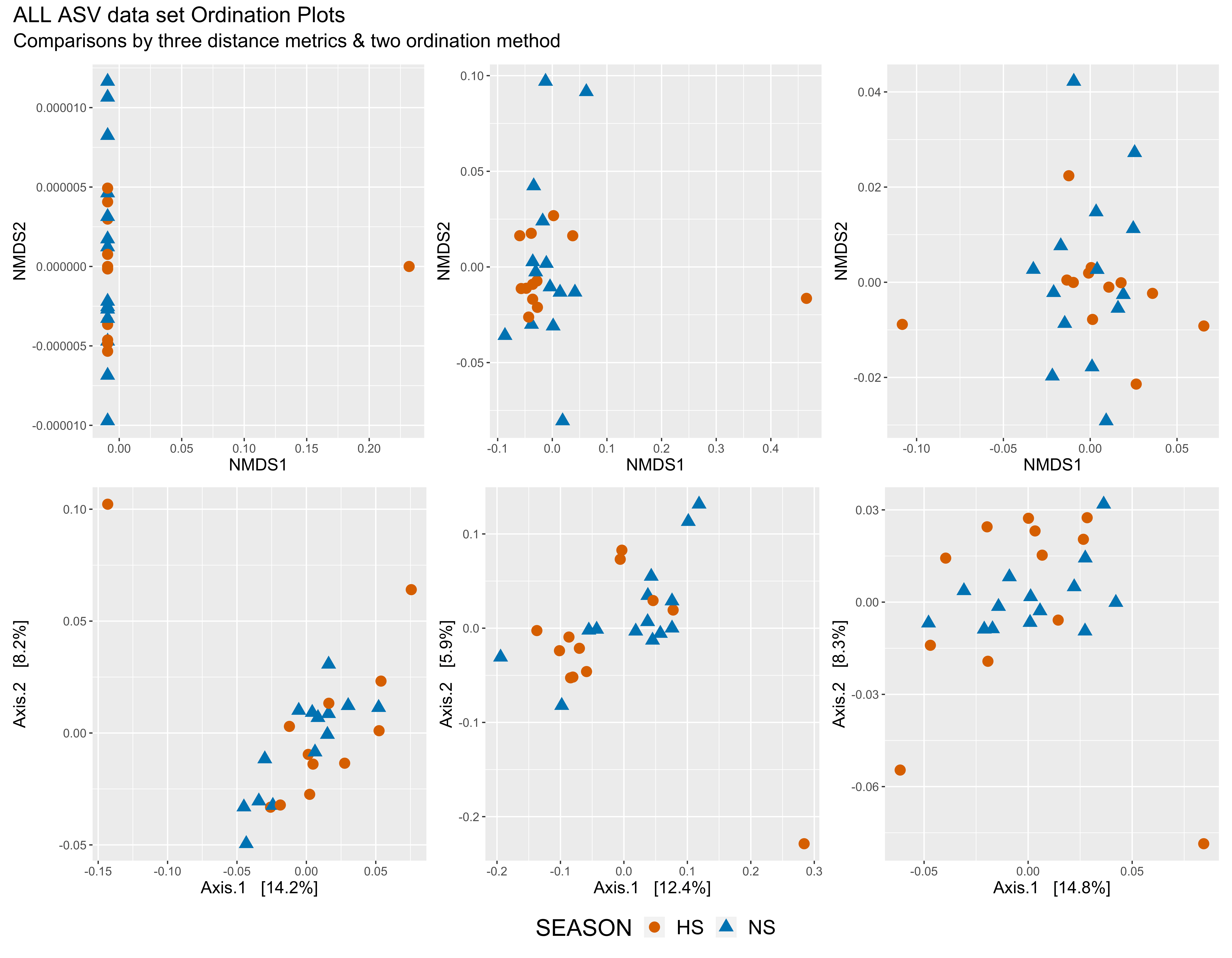
Figure 15: Left = Jensen-Shannon Divergence, middle = UniFrac (unwieghted), right = UniFrac (wieghted); Top = NMDS, bottom = PCoA.
Punta Caracol (outer bay)
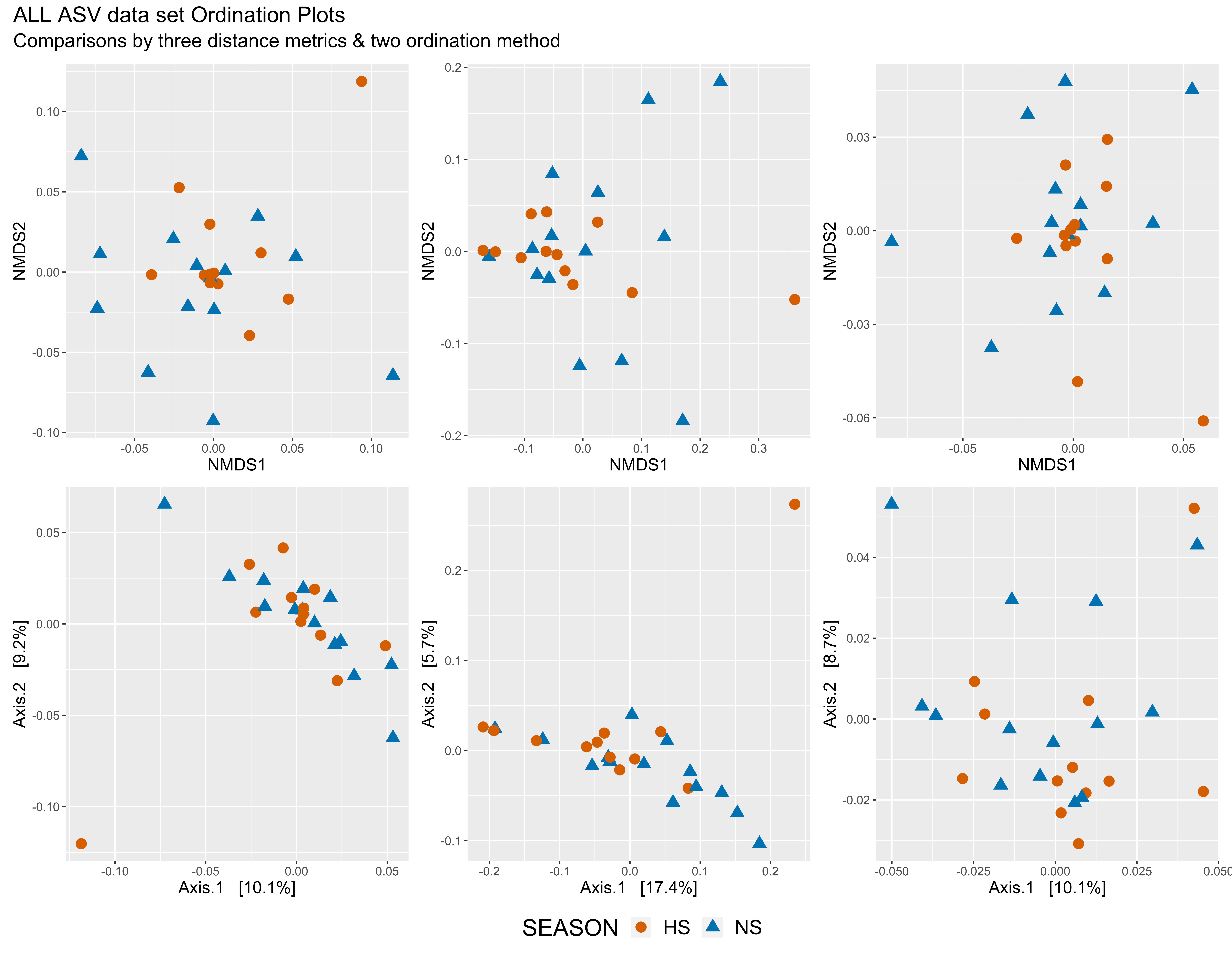
Figure 16: Left = Jensen-Shannon Divergence, middle = UniFrac (unwieghted), right = UniFrac (wieghted); Top = NMDS, bottom = PCoA.
Plots PIME ASVs
remove(list = ls())
ssu_ps_pime_merge_ALMR <- readRDS("files/trepo/pime/rdata/ssu_ps_merge_asv_pime_ALMR.rds")
ssu_ps_pime_merge_CRIS  <- readRDS("files/trepo/pime/rdata/ssu_ps_merge_asv_pime_CRIS.rds")
ssu_ps_pime_merge_PAST <- readRDS("files/trepo/pime/rdata/ssu_ps_merge_asv_pime_PAST.rds")
ssu_ps_pime_merge_PUCL <- readRDS("files/trepo/pime/rdata/ssu_ps_merge_asv_pime_PUCL.rds")
objects()
Before we begin, we must first transform sample counts to relative abundance for both data sets.
samp_ps <- c("ssu_ps_pime_merge_ALMR", "ssu_ps_pime_merge_CRIS", "ssu_ps_pime_merge_PAST", "ssu_ps_pime_merge_PUCL")
for (i in samp_ps) {
     tmp_name <- purrr::map_chr(i, ~ paste0(., "_prop"))
     tmp_get <- get(i)
     tmp_ps <- transform_sample_counts(tmp_get, function(otu) otu/sum(otu))
     tmp_ps@phy_tree <- NULL
     tmp_ps <- prune_samples(sample_sums(tmp_ps) > 0, tmp_ps)
     tmp_tree <- rtree(ntaxa(tmp_ps), rooted = TRUE, tip.label = taxa_names(tmp_ps))
     tmp_ps <- merge_phyloseq(tmp_ps, sample_data, tmp_tree)
     print(tmp_name)
     assign(tmp_name, tmp_ps)
     rm(list = ls(pattern = "tmp_"))
}
samp_ps <- c("ssu_ps_pime_merge_ALMR", "ssu_ps_pime_merge_CRIS", "ssu_ps_pime_merge_PAST", "ssu_ps_pime_merge_PUCL")
dist <- c("wunifrac", "unifrac", "jsd")
for (i in samp_ps){
for (d in dist){
tmp_name <- purrr::map_chr(d, ~ paste0(i, "_dist_", .))
tmp_name_plot <- purrr::map_chr(d, ~ paste0(i, "_dist_", ., "_plot"))
tmp_get <- get(purrr::map_chr(i, ~ paste0(., "_prop")))
ord_meths <- c("NMDS", "PCoA", "CCA", "DCA") # MDS = PCoA, "CCA", "DCA", "DPCoA", "RDA"
tmp_plist_name <- purrr::map_chr(d, ~ paste0(i, "_", ., "_plist"))
tmp_plist <- llply(as.list(ord_meths), function(i, physeq, d) {
ordi = ordinate(physeq, method = i, distance = d)
plot_ordination(physeq, ordi, "samples", color = "SEASON")
}, tmp_get, d)
names(tmp_plist) <- ord_meths
tmp_df <- ldply(tmp_plist, function(x){
df = x$data[, 1:2]
colnames(df) = c("Axis_1", "Axis_2")
return(cbind(df, x$data))})
names(tmp_df)[1] = "method"
## NEXT LINE REORDER FACTORS
tmp_df$SITE <- factor(tmp_df$SITE, levels = c("ALMR", "PAST", "CRIS", "PUCL"))
tmp_plot <- ggplot(tmp_df, aes(Axis_1, Axis_2,
color = SEASON, shape = SEASON, fill = SEASON))
tmp_plot <- tmp_plot + geom_point(size = 2)
tmp_plot <- tmp_plot + facet_wrap(~method, scales = "free")
tmp_plot <- tmp_plot + scale_colour_manual(values = swel_col)
assign(tmp_plist_name, tmp_plist)
assign(tmp_name, tmp_df)
assign(tmp_name_plot, tmp_plot)
rm(list = ls(pattern = "tmp_"))
}
}
objects(pattern = "_dist_")
objects()plist_name <- objects(pattern="_plist")
plot_num <- c(1,2)
for (i in plist_name) {
for (j in plot_num) {
tmp_get_i <- get(i)
## NEXT LINE REORDER FACTORS
tmp_get_i[[j]]$data$SITE <- factor(tmp_get_i[[j]]$data$SITE,
levels = c("ALMR", "PAST", "CRIS", "PUCL"))
tmp_ord <- names(tmp_get_i)[j]
tmp_name <- stringr::str_replace(i, "plist", tmp_ord)
tmp_plot <- tmp_get_i[[j]] + scale_colour_manual(values = swel_col)
tmp_plot <- tmp_plot + geom_point(size = 4, aes(shape = SEASON)) +
theme(legend.position = "bottom")
tmp_plot$labels$shape <- "SEASON"
assign(tmp_name, tmp_plot)
rm(list = ls(pattern = "tmp_"))
}
}Almirante (inner bay)
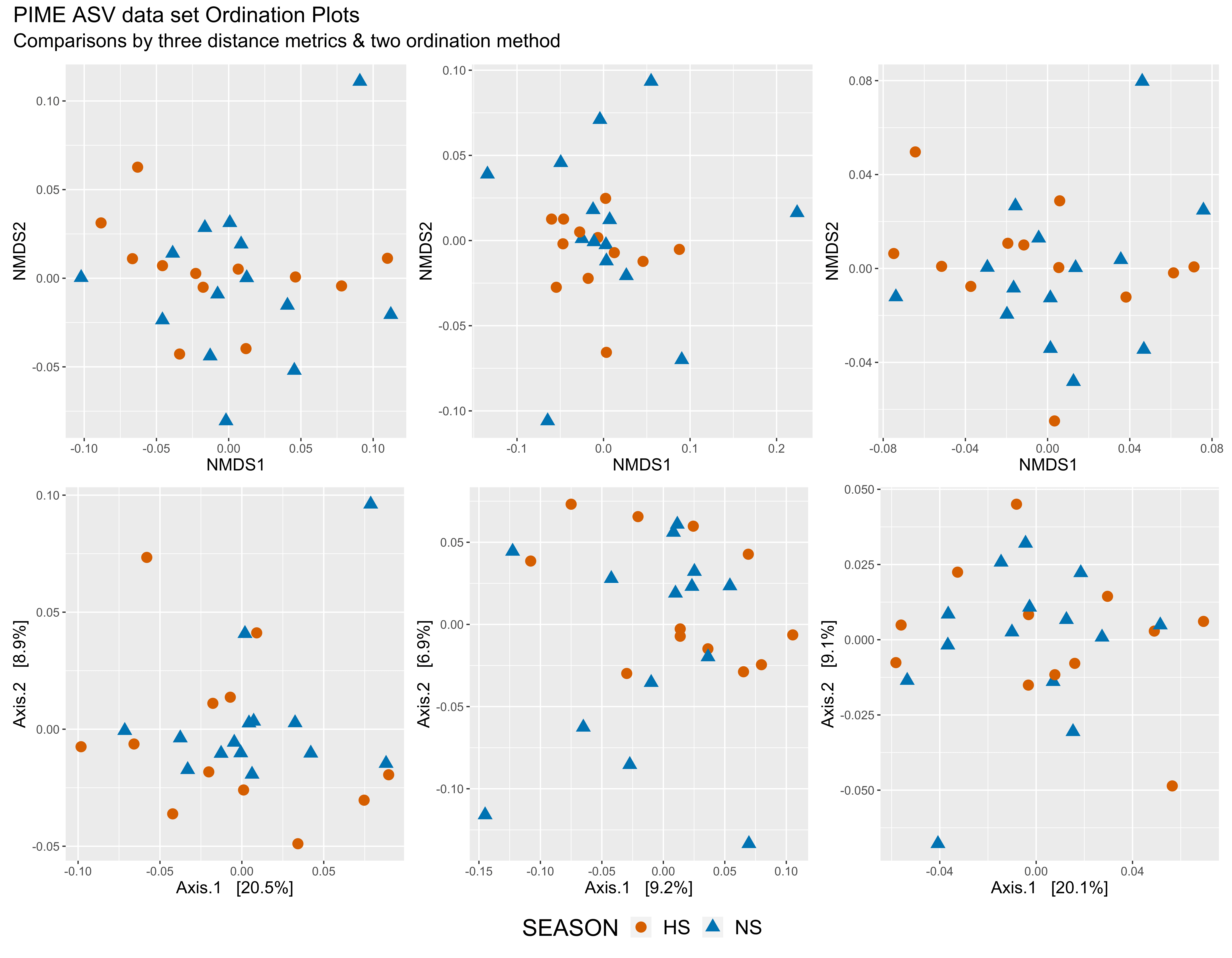
Figure 17: Left = Jensen-Shannon Divergence, middle = UniFrac (unwieghted), right = UniFrac (wieghted); Top = NMDS, bottom = PCoA.
Pastores (inner bay)
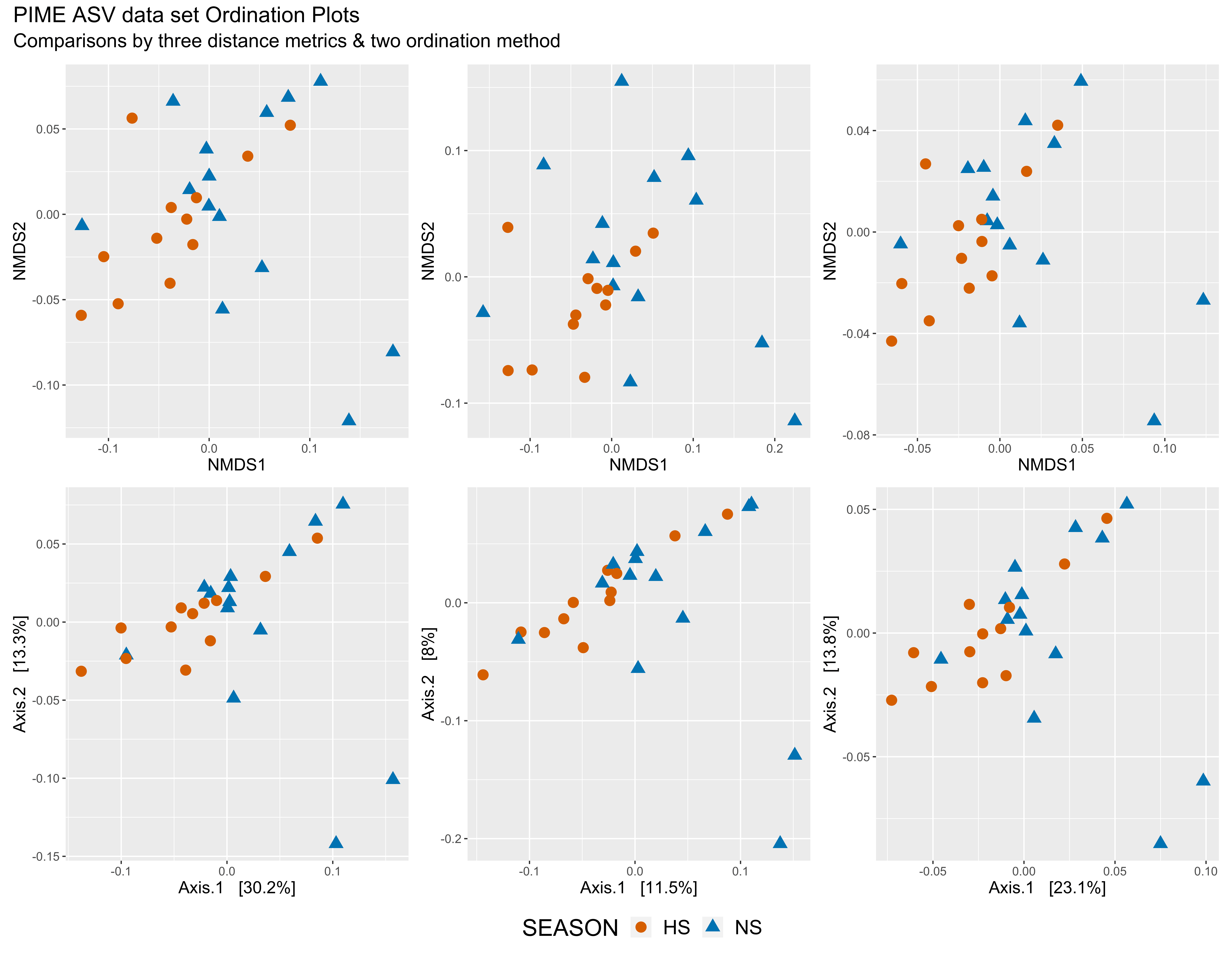
Figure 18: Left = Jensen-Shannon Divergence, middle = UniFrac (unwieghted), right = UniFrac (wieghted); Top = NMDS, bottom = PCoA.
Cristobal (outer bay)
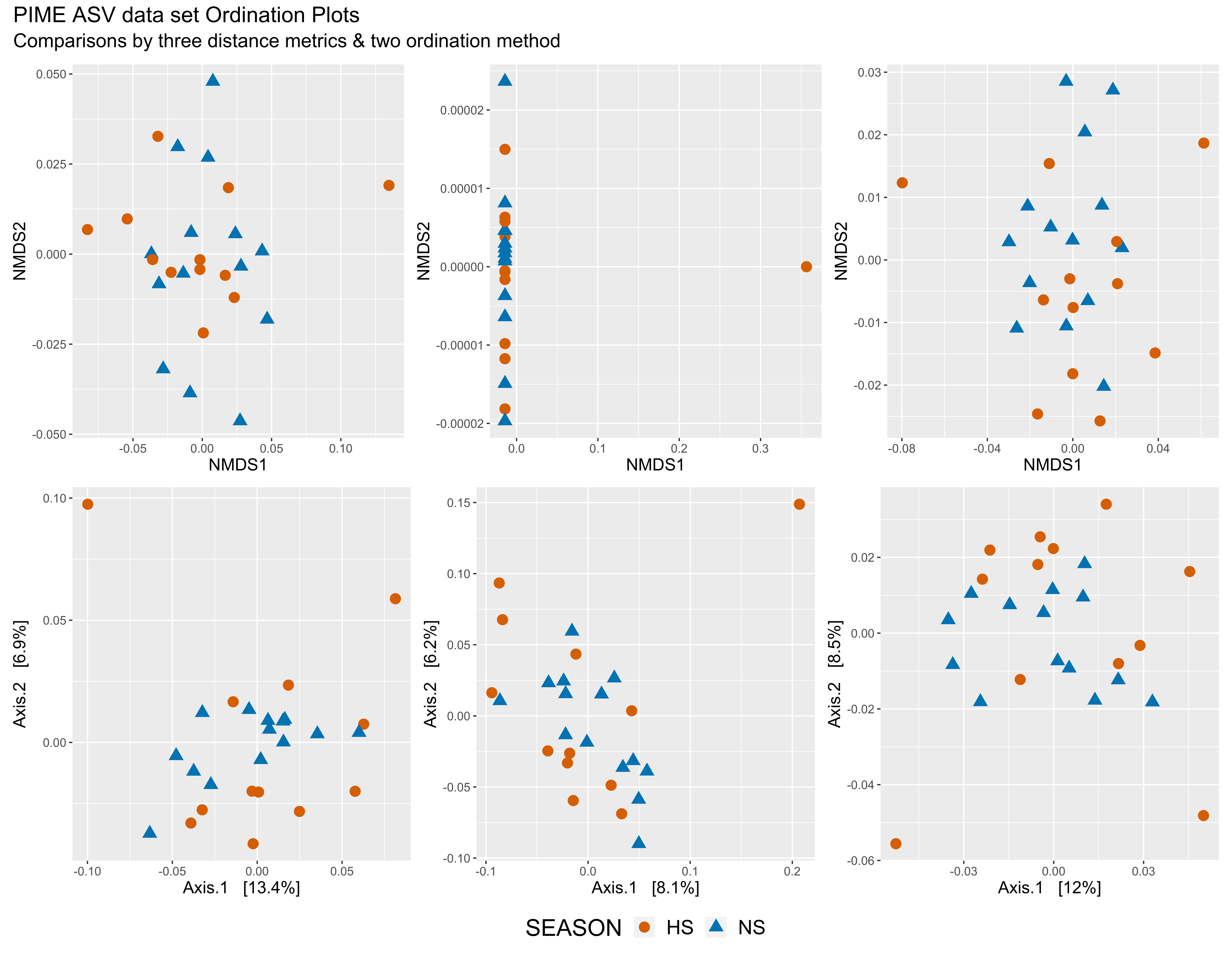
Figure 19: Left = Jensen-Shannon Divergence, middle = UniFrac (unwieghted), right = UniFrac (wieghted); Top = NMDS, bottom = PCoA.
Punta Caracol (outer bay)
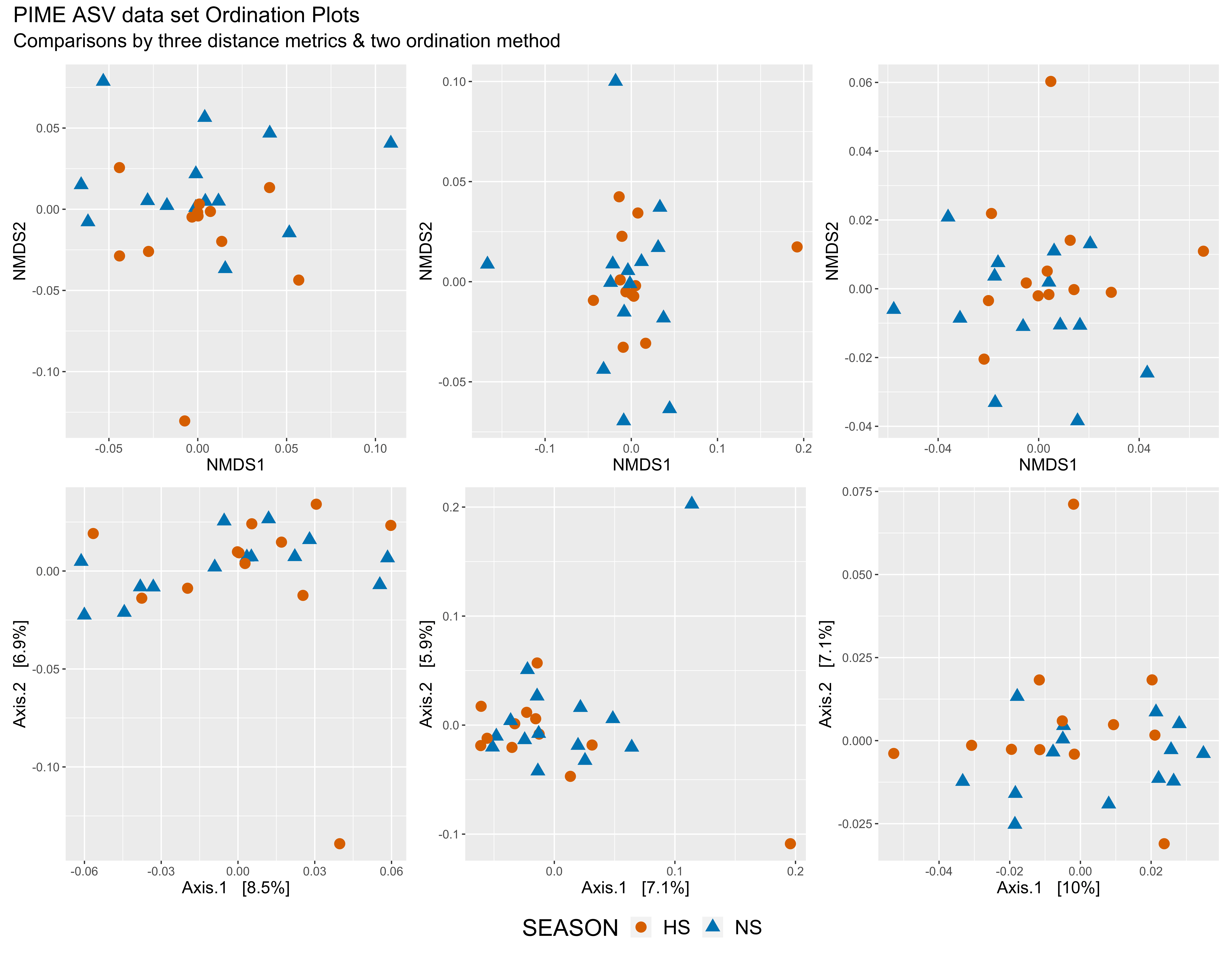
Figure 20: Left = Jensen-Shannon Divergence, middle = UniFrac (unwieghted), right = UniFrac (wieghted); Top = NMDS, bottom = PCoA.
Source Code
The source code for this page can be accessed on GitHub by clicking this link. Please note, that in order to process the data and build the website, we needed to run the workflow and get the results. Then hard code the results and turn off the individual commands. So the raw file for this page is a bit messy—you have been warned.